Applying and tuning a quantile random forest regression model

[nikos_geo]

I have a data.frame with 1 response variable, called ntl, and 11 predictors. My goal is to predict the the response using quantile random forest (QRF) regression. Why QRF and not simple RF? Well, the
response variable is the nighttime light which means in my study area (map 3, called Reference ntl, shown below) there are some bright areas (highlighted in red squares). Prediction with "classical" RF tends to underestimate these bright areas (conditional bias). I thought that by using QRF I could "enhance" the bright spots (i.e., give more weight to the outliers, or the brighter areas) when predicting ntl.

Before I come to this conclusion, I splitted my data.frame using using a stratified strategy in case I could get reasonable regression results using RF (much like this example). After predicting using the test set, I used the model created from the training set, to the whole dataset and I plotted the residuals from the whole dataset as a raster layer (I created a map). The residuals map is shown below:

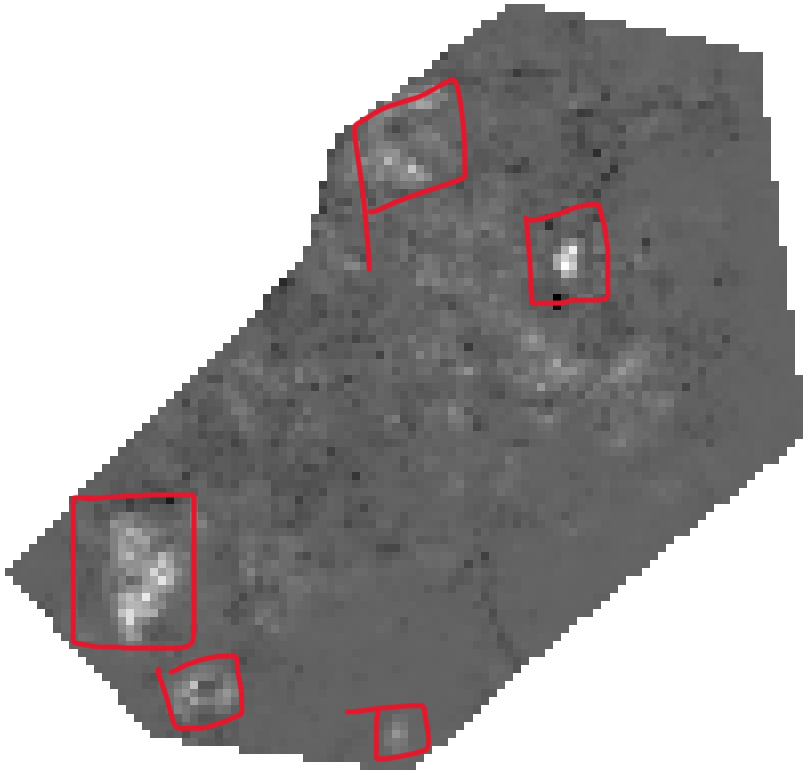
Figure of the RF residuals using the whole dataset.

For comparison, this is the reference ntl image:

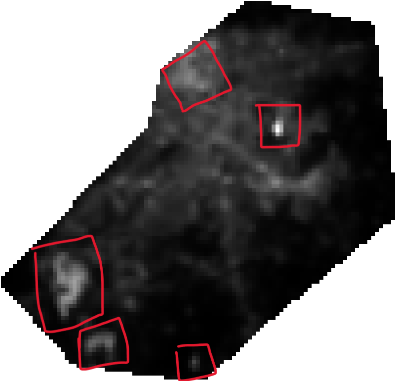
Reference ntl.

As you can see:

1. there is a spatial structure in the residuals, especially around the bright areas (highlighted in red). This means that:
   1.1. The RF model can not model well enough the extreme values.
   1.2. For a "good" model I would expect to see a random pattern in the residuals image. This can also be seen from the plot of fitted vs residuals values, shown below:

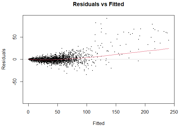
Plot of residuals vs fitted.

Lastly, I have to mention that I tried several tuning strategies for the RF model, that is, I increased the number of trees (up to 10001), I tuned the mtry and min_n parameters) but the results were no better. Based on these results I concluded that I might need a model that can weight more the extreme values (i.e., the bright areas in the image or the the large values in the data.frame) in order to capture the variability of the response, meaning, it will map the bright areas accuretelly.

I have conducted some explanatory spatial data analysis (ESDA) so that I could understand the data a bit better. Below, is the histogram of the response variable. Clearly, there distribution is right skewed (and possibly there is bimodality?)

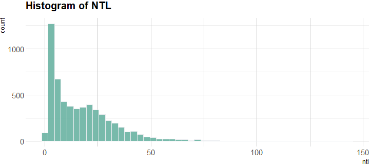
Histogram of the response variable (ntl).

Moreover, I created a boxplot of the response to further illustrate the outliers (bright areas).

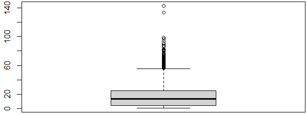
Boxplot of the response variable (ntl).

Next, I created scatter plots showing the response (y-axis) and the predictors (x-axis) in order to see the relationships. As expected, the ntl are positively correlated with the population (pop), the built-up indices (agbh, ndbi, ebbi, nbai), the land surface temperature (tirs), the road density (road), and a spectral band (pan), while the ntl is negatively correlated with the near-infrared (nir), which makes sense because the nir band is associated with the vegetation.

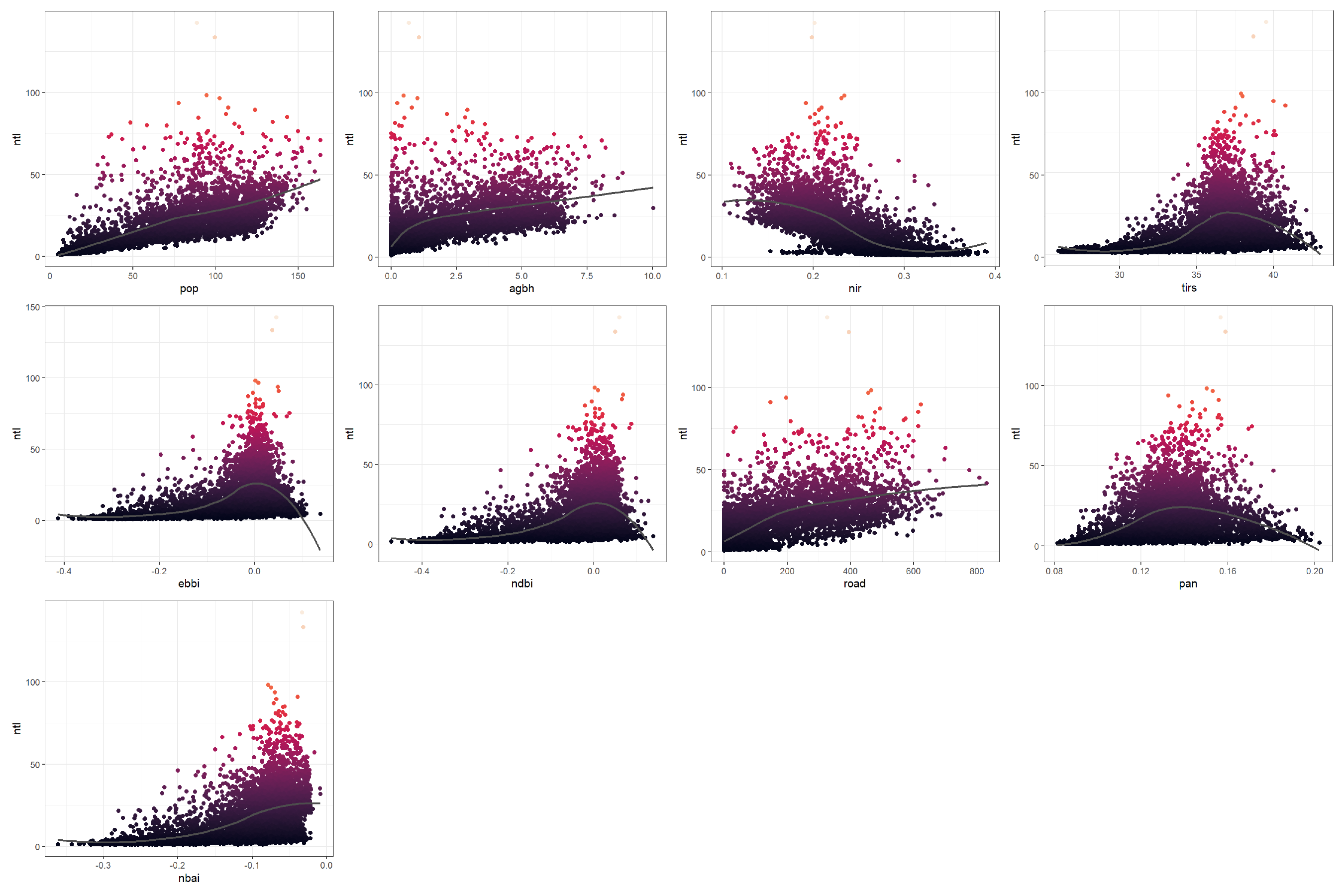
Scatterplots of the response vs predictors.

I am very new to tidymodels (working with the package only recently) so any help would be nice:

1. if I could use the tidymodels + ranger packages to perform quantile random forest regression (I know that the ranger package alone has the choice quantreg in the function ranger and you can specify the desired quantiles, for example, 0.75, 0.8 etc).
2. if so, how should I proceed? In the link I shared above, the author is using the "classical" RF (using the ranger package). What about fine-tuning of the hyperparameters when using QRF? Should I follow the "usual" hyperparameter tuning strategies? By usual I mean, the steps in the shared link (mtry and min_n). I know for a fact that for QRF I need more trees (ntrees) than the RF, the recommended value for the former is 2000. If for example, I want to make predictions using the 75th quantile, how should I tune the model for that specific quantile?

I apologize for the long post but I this issue troubles me for several months now and I need some guidance/help. The data.frame I am using has several thousands rows so you can dowload it from here.

Do not worry though, when using RF the whole process (tuning, applying the model and predicting) takes about 4-5 minutes on my laptop.

Below is one of my tries using RF:

wd <- "path/"

# this is the CRS
provoliko <- "EPSG:24313"

df <- read.csv(paste0(wd, 'block.data.csv'))

# extract the x and y (coordinates) columns from the data.frame
crds <- df[, 1:2]

keep <- c("ntl", "pop", "agbh", "nir",  "lu", "ebbi", "ndbi", "road", "pan", "nbai", 
          "tirs")
df <- df[keep]

library(tidymodels)
set.seed(456)

ikea_split <- initial_split(df, strata = ntl, prop = 0.80)
ikea_train <- training(ikea_split)
ikea_test <- testing(ikea_split)

set.seed(567)
ikea_folds <- bootstraps(ikea_train, strata = ntl)
ikea_folds

library(usemodels)
eq1 <- ntl ~ .
use_ranger(eq1, data = ikea_train)

library(textrecipes)
ranger_recipe <-
  recipe(formula = eq1, data = ikea_train)

ranger_spec <-
  rand_forest(mtry = tune(), min_n = tune(), trees = 501) %>%    # 1001 trees
  set_mode("regression") %>%
  set_engine("ranger")

ranger_workflow <-
  workflow() %>%
  add_recipe(ranger_recipe) %>%
  add_model(ranger_spec)

set.seed(678)
doParallel::registerDoParallel()
ranger_tune <-
  tune_grid(ranger_workflow,
            resamples = ikea_folds,
            grid = 10                 # 10
)

show_best(ranger_tune, metric = "rsq")

autoplot(ranger_tune)

final_rf <- ranger_workflow %>%
  finalize_workflow(select_best(ranger_tune, metric = "rsq"))

final_rf

ikea_fit <- last_fit(final_rf, ikea_split)
ikea_fit

collect_metrics(ikea_fit)

collect_predictions(ikea_fit) %>%
  ggplot(aes(ntl, .pred)) +
  geom_abline(lty = 2, color = "gray50") +
  geom_point(alpha = 0.5, color = "midnightblue") +
  coord_fixed()

predict(ikea_fit$.workflow[[1]], ikea_test[15, ])

ikea_all <- predict(ikea_fit$.workflow[[1]], df[, 2:11])
ikea_all <- as.data.frame(cbind(df$ntl, ikea_all))
ikea_all$rsds <- ikea_all$`df$ntl` - ikea_all$.pred
ikea_all <- as.data.frame(cbind(crds, ikea_all))
ikea_all <- ikea_all[,-3:-4]

library(terra)

rsds <- rast(ikea_all, type = "xyz")
crs(rsds) <- provoliko
writeRaster(rsds, paste0(wd, "rf_resids.tif"), overwrite = TRUE)

library(vip)

imp_spec <- ranger_spec %>%
  finalize_model(select_best(ranger_tune, metric = "rsq")) %>%
  set_engine("ranger", importance = "permutation")

workflow() %>%
  add_recipe(ranger_recipe) %>%
  add_model(imp_spec) %>%
  fit(ikea_train) %>%
  extract_fit_parsnip() %>%
  vip(aesthetics = list(alpha = 0.8, fill = "midnightblue"))