Appending a robvis traffic-light plot to a meta::forest plot using gridExtra: is there a way of reducing the size of the robvis plot?

[mmsj]

I am using the robvis development version to create an RoB2 traffic-light plot that I would like to add to my meta-forest plot. However, I am unable to prevent the RoB plot bottom legends ("Domains" and "Judgement") from overlapping. Is there a way around this please? Or is there a way of reducing the overall size of the traffic-light plot so that it fits better next to the forest plot.

Code and plot as follows.

 library(meta)
    # metabin data
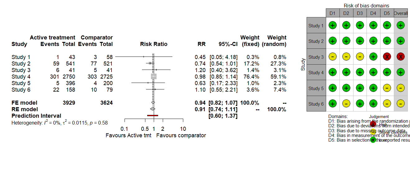
    dat <- data.frame(Study_name = c("Study 1", "Study 2", "Study 3", "Study 4", "Study 5", "Study 6"),
                    Tmt_D =c(1, 59, 6, 301, 5, 22),Tmt_T =c(43, 541, 41, 2750, 396, 158),
                    Con_D =c(3, 77, 5, 303, 4, 10),Con_T =c(58, 521, 41, 2725, 200, 79),
     # RoB2 data
     rob <- data.frame(Study_name = c("Study 1", "Study 2", "Study 3", "Study 4", "Study 5", "Study 6"),
                    D1 = c("Low", "Low", "Some concerns", "Low", "Low", "Low"),
                    D2 = c("Low", "Low", "Some concerns", "Low", "Low", "Some concerns"),
                    D3 = c("Low", "Low", "Some concerns", "Low", "Low", "Low"),
                    D4 = c("Low", "Low", "Low", "Low", "Low", "Low"),
                    D5 = c("Low", "Low", "High", "Low", "Some concerns", "Some concerns"),
                    Overall = c("Low", "Low", "High", "Low", "Some concerns", "Some concerns"))
    # run binary meta-analysis
    bin.1 <- metabin(event.e=Tmt_D, n.e=Tmt_T, event.c=Con_D, n.c=Con_T, 
                 studlab=Study_name,data= dat,method="inverse",sm="RR",
                 prediction=TRUE)

    # create binary forest plot as ggplot
    library(ggplotify)
    p1 <- as.ggplot(~forest(bin.1, text.common = "FE model", text.random = "RE model",
                text.predict = "Prediction Interval", text.w.common = "fixed",
                text.w.random = "random",label.e = "Active treatment", 
                label.c = "Comparator", label.right = "Favours comparator", 
                label.left = "Favours Active tmt"))
    # create robvis RoB2 plot
    library(robvis)
    p2 <- rob_traffic_light(rob, psize = 8, tool = "ROB2")

    # append RoB2 plot to forest plot
    library(gridExtra)
    grid.arrange(p1, p2, widths=c(8,3), heights=c(35,5))