Annotate ggplot2 with regression equation and r squared

Hi there,

I would like to annotate ggplot2 with a regression equation and r squared. Ideally, it would work for facets and the location of the annotation could be conveniently specified (e.g. "topleft"). Maybe it’s just my ignorance but there seems to be no specific function in ggplot2 package to achieve this. This is surprising to me because displaying r squared, slope and intercept in the plot is quite common and informative. Having the option to display model coefficients and R2 as plot annotation would be a great extension of geom_smooth() or stat_smooth() functions, even if it worked for lm method only.

I found the following answers to a similar question on Stack Overflow and RPubs, but the solutions are not so straightforward (problems with facets, positioning).

https://stackoverflow.com/questions/7549694/adding-regression-line-equation-and-r2-on-graph
https://rstudio-pubs-static.s3.amazonaws.com/213536_d4b3975ee92b43af8671057ccefb90c7.html

Do you guys have any recommendations of how to add model information to the plot?

Many thanks!

2 Likes

Are you able to make a reprex for this? Even if it's just showing us your plotting code with some dummy data :slight_smile:

Have you tried the stat_poly_eq() function in the ggpmisc package?

1 Like

The ggpmisc package looks interesting and probably does what you want.

Nevertheless, to my knowledge the ggplot2 function geom_smooth() returns predictions from the model, but not the model object itself. So getting the r squared, slope and intercept out from that isn't going to work.

Similar to your links I have seen people call a lm() function and then pass the values in. For example, Susan Johnston has this ggplotRegression function which is quite nice which I'll reproduce here. It works fine for single graphs:

ggplotRegression <- function(fit){

require(ggplot2)

ggplot(fit$model, aes_string(x = names(fit$model)[2], y = names(fit$model)[1])) + 
  geom_point() +
  stat_smooth(method = "lm", col = "red") +
  labs(title = paste("Adj R2 = ",signif(summary(fit)$adj.r.squared, 5),
                     "Intercept =",signif(fit$coef[[1]],5 ),
                     " Slope =",signif(fit$coef[[2]], 5),
                     " P =",signif(summary(fit)$coef[2,4], 5)))
}

ggplotRegression(lm(Sepal.Length ~ Petal.Width, data = iris))

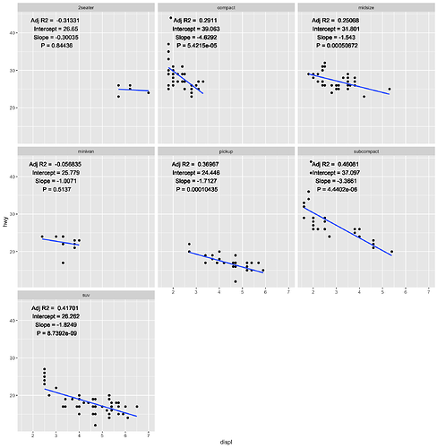
To do this for facets you could do something like this:

mpg %>% 
  nest(-drv) %>% 
  mutate(model = map(data, ~ lm(hwy~displ, data = .x)),
         adj.r.squared = map_dbl(model, ~ signif(summary(.x)$adj.r.squared, 5)),
         intercept = map_dbl(model, ~ signif(.x$coef[[1]],5)),
         slope = map_dbl(model, ~ signif(.x$coef[[2]], 5)),
         pvalue = map_dbl(model, ~ signif(summary(.x)$coef[2,4], 5)) 
         ) %>% 
  select(-data, -model) %>% 
  left_join(mpg) %>% 
  
  ggplot(aes(displ, hwy)) +
  geom_point() +
  geom_smooth(se = FALSE, method = "lm") +
  facet_wrap(~drv) +
  geom_text(aes(3, 40, label = paste("Adj R2 = ", adj.r.squared, "\n",
                                   "Intercept =",intercept, "\n",
                                   "Slope =", slope, "\n",
                                   "P =", pvalue)))

But you have to manually adjust position etc. I'm sure this could be generalised.

1 Like

We have a ready-made plot of a similar nature.

Plot a scatter plot with marginals. — ScatterHist • WVPlots

2 Likes

Thanks for your reply! It's very useful.

I tried to rewrite the code to create functions that would take data, xvar, yvar and group (for faceting) as arguments. However, there is something wrong with my syntax in both examples.

  1. single graph example
ggplotRegression <- function(dat, xvar, yvar){
  
  require(ggplot2)
  
  fit <- lm(yvar~xvar, dat)
  
  ggplot(fit$model, aes_string(x = names(fit$model)[2], y = names(fit$model)[1])) + 
    geom_point() +
    stat_smooth(method = "lm", col = "red") +
    labs(title = paste("Adj R2 = ",signif(summary(fit)$adj.r.squared, 5),
                       "Intercept =",signif(fit$coef[[1]],5 ),
                       " Slope =",signif(fit$coef[[2]], 5),
                       " P =",signif(summary(fit)$coef[2,4], 5)))
}
ggplotRegression(Sepal.Length, Petal.Width, iris)
  1. facet graph example
library(tidyverse)

facetRegression <- function(dat, xvar, yvar, group) {
  xvar <- enquo(xvar)
  yvar <- enquo(yvar)
  group <- enquo(group)
  
  dat %>% 
    nest(-!!group) %>% 
    mutate(model = map(data, ~ lm(!!xvar~!!yvar, data = .x)),
           adj.r.squared = map_dbl(model, ~ signif(summary(.x)$adj.r.squared, 5)),
           intercept = map_dbl(model, ~ signif(.x$coef[[1]],5)),
           slope = map_dbl(model, ~ signif(.x$coef[[2]], 5)),
           pvalue = map_dbl(model, ~ signif(summary(.x)$coef[2,4], 5)) 
    ) %>% 
    select(-data, -model) %>% 
    left_join(dat) %>% 
    
    ggplot(aes_(substitute(xvar), substitute(yvar))) +
    geom_point() +
    geom_smooth(se = FALSE, method = "lm") +
    facet_wrap(~!!group) +
    geom_text(aes(3, 40, label = paste("Adj R2 = ", adj.r.squared, "\n",
                                       "Intercept =",intercept, "\n",
                                       "Slope =", slope, "\n",
                                       "P =", pvalue)))
}
facetRegression(mpg, displ, hwy, drv)

These are probably very naive attempts, but I'm not very experienced in writing functions. In the past, I wrote some non-elegant functions in base R but after switching to tidyverse I got confused with tidy evaluation, so now I'm not even sure where I need to use it and where I'm fine with the standard way of writing function (I think I don't need the tidy eval in the single graph example, right?).

There is clearly something wrong in the way I specify the model equation within both functions. I tried to write the equation in a couple of different ways, e.g.,

lm(yvar~xvar, dat)

with(dat, lm(yvar~xvar)) 

lm(dat[[yvar]]~dat[[xvar]])

...but no success :frowning:

For the facet example, I also tried to separate the code into two steps i) data preparation and ii) ggplot plotting, but was not able to get the function working properly for either piece of the code.

I thought about the strategy for positioning the text in each facet. I think it should be possible to get ymax and xmin for each drv group in the data preparation phase and then use it with some reasonable offset within geom_text(), but typing the correct syntax it is clearly beyond my current programming skills :wink:

I would appreciate help with the code above, but I would be extremely grateful for some "philosophical" discussion on how to approach building functions like these step by step. I don't have CS background (I come from the field of biology) and use R to analyze my biological data. I often find myself in the situation when I get some analyses and graphs done, but as the project grows I start to get lost in my code. I try to simplify it (e.g., by writing a function) but then get stuck at some programming obstacle. I then spend a lot of time fiddling with the code and often don't get over the obstacle because I cannot come up with the right syntax. I guess my problem is that I want to achieve too complex things for my level of programming skills, but how do I know what's the right level of complexity is. I want to be falling in the pit of programming success :slight_smile:

Is there any specific reason you want to use non-standard evaluation for this? With strings your first example is straightforward:

library(tidyverse)

ggplotRegression <- function(dat, xvar, yvar){
  
  fml <- paste(yvar, "~", xvar)

  fit <- lm(fml, dat)
  
  ggplot(fit$model, aes_string(x = names(fit$model)[2], y = names(fit$model)[1])) + 
    geom_point() +
    stat_smooth(method = "lm", col = "red") +
    labs(title = paste("Adj R2 = ",signif(summary(fit)$adj.r.squared, 5),
                       "Intercept =",signif(fit$coef[[1]],5 ),
                       " Slope =",signif(fit$coef[[2]], 5),
                       " P =",signif(summary(fit)$coef[2,4], 5)))
}
ggplotRegression(iris, "Sepal.Length", "Petal.Width")

Many thanks for the solution! No, there's no specific reason to use NSE and I supposed I won't need it for the first example. Just couldn't come up with a syntax that would work, although I spend two evenings on this :slight_smile:
With the second example with facets, I cannot get by without NSE, right?

Yes, you can :slight_smile:

library(tidyverse)

facetRegression <- function(dat, xvar, yvar, group) {
  fml <- paste(yvar, "~", xvar)
  
  group <- rlang::sym(group)
  wrap_fml <- rlang::new_formula(rhs = group, lhs = NULL)
  dot <- rlang::quo(-!!group)
  
  dat %>% 
    nest(!!dot) %>% 
    mutate(model = map(data, ~ lm(fml, data = .x)),
           adj.r.squared = map_dbl(model, ~ signif(summary(.x)$adj.r.squared, 5)),
           intercept = map_dbl(model, ~ signif(.x$coef[[1]],5)),
           slope = map_dbl(model, ~ signif(.x$coef[[2]], 5)),
           pvalue = map_dbl(model, ~ signif(summary(.x)$coef[2,4], 5)) 
    ) %>% 
    select(-data, -model) %>% 
    left_join(dat) %>% 
    
    ggplot(aes_string(xvar, yvar)) +
    geom_point() +
    geom_smooth(se = FALSE, method = "lm") +
    facet_wrap(wrap_fml) +
    geom_text(aes(3, 40, label = paste("Adj R2 = ", adj.r.squared, "\n",
                                       "Intercept =",intercept, "\n",
                                       "Slope =", slope, "\n",
                                       "P =", pvalue)))
}
facetRegression(mpg, "displ", "hwy", "class")
8 Likes

Awesome! Thanks for the elegant solution. For the time being, I added x.pos and y.pos arguments and adjust the geom_text() position manually for different plots.

4 Likes

also you can try:

geom_text(x=-Inf,y=+Inf,hjust="inward") to position text on top left and have the text go into the center of the plot regardless of current facet limits.

Neat trick with the Infs. Thanks for your advice! I used geom_text(aes(x=-Inf, y=Inf, hjust=0, vjust=1, label=...) and that worked great.

A post was split to a new topic: help adding annotation to ggplot