Hello everyone,
I have encountered a situation with two rasters that have the same projection, although the full description returned by terra::crs() appears to be different. Notably, raster1 has a coarser resolution and a larger extent compared to raster2. My goal is to align the extent of raster1 with that of raster2.
Despite the differences in the description of the CRS, the crucial aspect seems to be that the projections match, which is fortunate.
Given that raster1 has a coarser resolution than raster2, I'm unable to directly employ the resample function. Therefore, my approach involved initially aggregating raster2 to match the resolution of raster1, and subsequently applying the resample function.
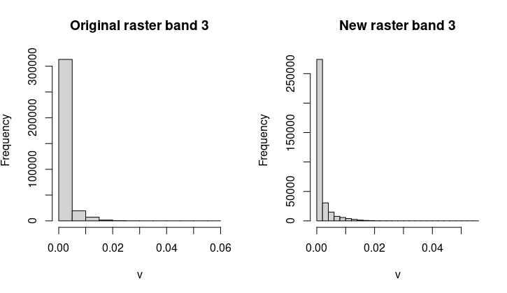
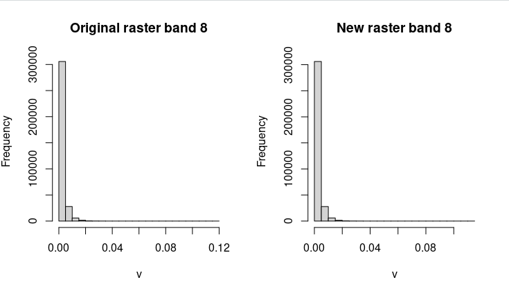
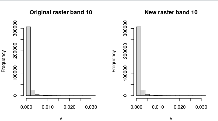
However, I have observed that the values of the resampled raster1 look notably different from the original raster1. This has raised concerns for me.
I'm seeking your insights on the following:
- Should I be concerned about the differences in values after resampling?
- What are your thoughts on my approach?
- Would you have taken a different approach?
I appreciate any advice or suggestions you may have regarding this matter. Thank you for your assistance!
I am posting here a reproducible code where I use the exact information of my original rasters including the different crs descriptions
library("purrr") # Data manipulation and functional programming tools
library("dplyr") # Data manipulation
#> Warning: il pacchetto 'dplyr' è stato creato con R versione 4.3.2
#>
#> Caricamento pacchetto: 'dplyr'
#> I seguenti oggetti sono mascherati da 'package:stats':
#>
#> filter, lag
#> I seguenti oggetti sono mascherati da 'package:base':
#>
#> intersect, setdiff, setequal, union
library("tmap") # Make map
#> Warning: il pacchetto 'tmap' è stato creato con R versione 4.3.2
#> The legacy packages maptools, rgdal, and rgeos, underpinning the sp package,
#> which was just loaded, will retire in October 2023.
#> Please refer to R-spatial evolution reports for details, especially
#> https://r-spatial.org/r/2023/05/15/evolution4.html.
#> It may be desirable to make the sf package available;
#> package maintainers should consider adding sf to Suggests:.
#> The sp package is now running under evolution status 2
#> (status 2 uses the sf package in place of rgdal)
#> Breaking News: tmap 3.x is retiring. Please test v4, e.g. with
#> remotes::install_github('r-tmap/tmap')
library("ggplot2") # Plot
#> Warning: il pacchetto 'ggplot2' è stato creato con R versione 4.3.3
library("sf") # Work with spatial data
#> Warning: il pacchetto 'sf' è stato creato con R versione 4.3.2
#> Linking to GEOS 3.11.2, GDAL 3.7.2, PROJ 9.3.0; sf_use_s2() is TRUE
library("terra")# Work with raster
#> terra 1.7.46
library("glue") # Work with strings
#>
#> Caricamento pacchetto: 'glue'
#> Il seguente oggetto è mascherato da 'package:terra':
#>
#> trim
raster1=rast()
crs(raster1)="GEOGCRS[\"unknown\",\n DATUM[\"World Geodetic System 1984\",\n ELLIPSOID[\"WGS 84\",6378137,298.257223563,\n LENGTHUNIT[\"metre\",1]],\n ID[\"EPSG\",6326]],\n PRIMEM[\"Greenwich\",0,\n ANGLEUNIT[\"degree\",0.0174532925199433],\n ID[\"EPSG\",8901]],\n CS[ellipsoidal,2],\n AXIS[\"longitude\",east,\n ORDER[1],\n ANGLEUNIT[\"degree\",0.0174532925199433,\n ID[\"EPSG\",9122]]],\n AXIS[\"latitude\",north,\n ORDER[2],\n ANGLEUNIT[\"degree\",0.0174532925199433,\n ID[\"EPSG\",9122]]]]"
ext(raster1)=c(-0.049999999152054, 359.949993895636, -90.05, 90.05)
res(raster1)=0.1
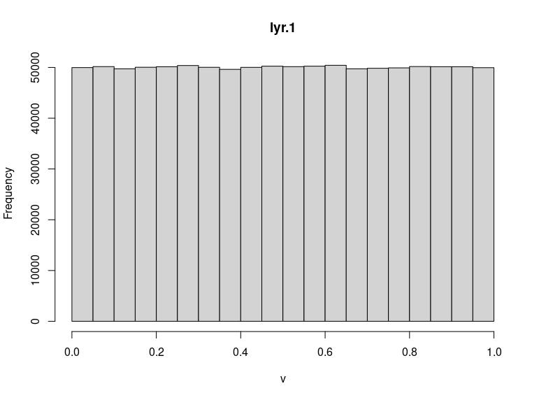
# Fill raster1 with random values
values(raster1) <- runif(ncell(raster1))
# Raster 2
raster2=rast()
crs(raster2)="GEOGCRS[\"WGS 84\",\n ENSEMBLE[\"World Geodetic System 1984 ensemble\",\n MEMBER[\"World Geodetic System 1984 (Transit)\"],\n MEMBER[\"World Geodetic System 1984 (G730)\"],\n MEMBER[\"World Geodetic System 1984 (G873)\"],\n MEMBER[\"World Geodetic System 1984 (G1150)\"],\n MEMBER[\"World Geodetic System 1984 (G1674)\"],\n MEMBER[\"World Geodetic System 1984 (G1762)\"],\n MEMBER[\"World Geodetic System 1984 (G2139)\"],\n ELLIPSOID[\"WGS 84\",6378137,298.257223563,\n LENGTHUNIT[\"metre\",1]],\n ENSEMBLEACCURACY[2.0]],\n PRIMEM[\"Greenwich\",0,\n ANGLEUNIT[\"degree\",0.0174532925199433]],\n CS[ellipsoidal,2],\n AXIS[\"geodetic latitude (Lat)\",north,\n ORDER[1],\n ANGLEUNIT[\"degree\",0.0174532925199433]],\n AXIS[\"geodetic longitude (Lon)\",east,\n ORDER[2],\n ANGLEUNIT[\"degree\",0.0174532925199433]],\n USAGE[\n SCOPE[\"Horizontal component of 3D system.\"],\n AREA[\"World.\"],\n BBOX[-90,-180,90,180]],\n ID[\"EPSG\",4326]]"
ext(raster2)=c(-180, 180, -90, 90)
res(raster2)=0.05
# Fill raster2 with random values
values(raster2) <- runif(ncell(raster2))
# Check if the rasters have the same CRS
if (crs(raster1, proj=TRUE) == crs(raster2,proj=TRUE)) {
print("The rasters have the same CRS")
} else {
print("The rasters have different CRS")
}
#> [1] "The rasters have the same CRS"
# Check if the rasters have the same extent
# Get the extents
extent1 <- ext(raster1)
extent2 <- ext(raster2)
# Compare the extents
if (extent1$xmin < extent2$xmin | extent1$xmax > extent2$xmax |
extent1$ymin < extent2$ymin | extent1$ymax > extent2$ymax) {
print("Raster 1 has a bigger extent")
} else if (extent1$xmin > extent2$xmin | extent1$xmax < extent2$xmax |
extent1$ymin > extent2$ymin | extent1$ymax < extent2$ymax) {
print("Raster 2 has a bigger extent")
} else {
print("Both rasters have the same extent")
}
#> [1] "Raster 1 has a bigger extent"
# Extent of ERA5 is bigger
print(extent1)
#> SpatExtent : -0.049999999152054, 359.950000000848, -90.05, 90.05 (xmin, xmax, ymin, ymax)
print(extent2)
#> SpatExtent : -180, 180, -90, 90 (xmin, xmax, ymin, ymax)
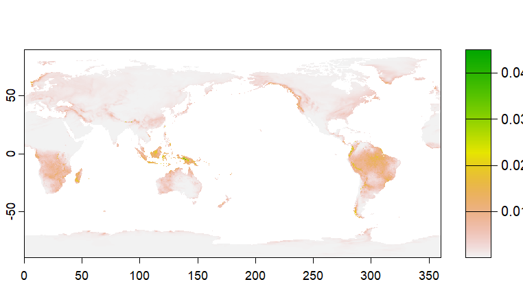
plot(raster2)

# Check if the rasters have the same resolution
if (res(raster1)[1] == res(raster2)[1]) {
print("The rasters have same resolution")
} else {
print("The rasters have different resolution")
}
#> [1] "The rasters have different resolution"
if (res(raster1)[1] > res(raster2)[1]) {
print("Raster 1 has a bigger cell size")
} else if (res(raster2)[1] > res(raster1)[1]) {
print("Raster 2 has a bigger cell size")
} else {
print("Both rasters have the same cell size")
}
#> [1] "Raster 1 has a bigger cell size"
res(raster1)
#> [1] 0.1 0.1
res(raster2)
#> [1] 0.05 0.05
# Resolution of raster1 is lower (coarser resolution)
# Thus change the resolution of raster 2.
raster2=aggregate(raster2,fact=2,fun=mean)
#> |---------|---------|---------|---------|=========================================
res(raster2)
#> [1] 0.1 0.1
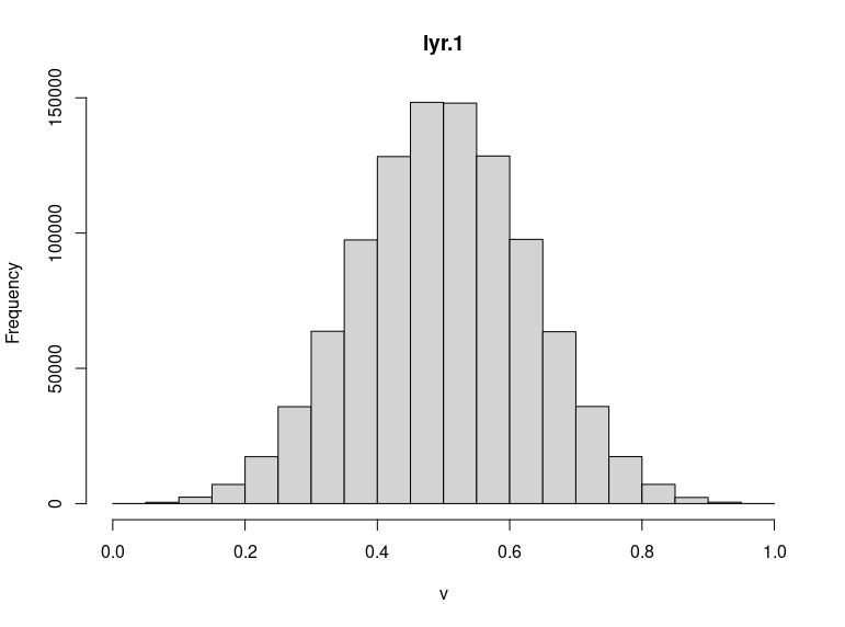
# Align the raster1 with the raster2 extent
raster1_resampled=resample(raster1,raster2,method="bilinear")
print(raster1_resampled)
#> class : SpatRaster
#> dimensions : 1800, 3600, 1 (nrow, ncol, nlyr)
#> resolution : 0.1, 0.1 (x, y)
#> extent : -180, 180, -90, 90 (xmin, xmax, ymin, ymax)
#> coord. ref. : +proj=longlat +datum=WGS84 +no_defs
#> source(s) : memory
#> name : lyr.1
#> min value : 0.01106466
#> max value : 0.98868102
print(raster1)
#> class : SpatRaster
#> dimensions : 1801, 3600, 1 (nrow, ncol, nlyr)
#> resolution : 0.1, 0.1 (x, y)
#> extent : -0.05, 359.95, -90.05, 90.05 (xmin, xmax, ymin, ymax)
#> coord. ref. : +proj=longlat +datum=WGS84 +no_defs
#> source(s) : memory
#> name : lyr.1
#> min value : 1.115259e-07
#> max value : 9.999999e-01