Adding forecast to line graph

[kuttan98]

Hi,
I have a data of growth rates year-wise. I want to get the forecast of growth for next 5 or 7 years. How can I do that?

library(tidyverse)
library(janitor)
library(readxl)

data<-tibble::tribble(
  ~year, ~growth,
  1990L,      7L,
  1991L,     10L,
  1992L,      5L,
  1993L,      7L,
  1994L,      8L,
  1995L,     10L,
  1996L,      4L,
  1997L,      7L,
  1998L,      5L,
  1999L,      5L,
  2000L,      8L,
  2001L,     10L,
  2002L,      9L,
  2003L,      8L,
  2004L,      5L,
  2005L,      6L,
  2006L,      9L,
  2007L,      9L,
  2008L,      5L
  )

data %>% 
  ggplot(aes(year,growth))+
  geom_line(size=2)+
  theme_minimal()

[technocrat]

# basic
library(forecast)
#> Registered S3 method overwritten by 'quantmod':
#>   method            from
#>   as.zoo.data.frame zoo
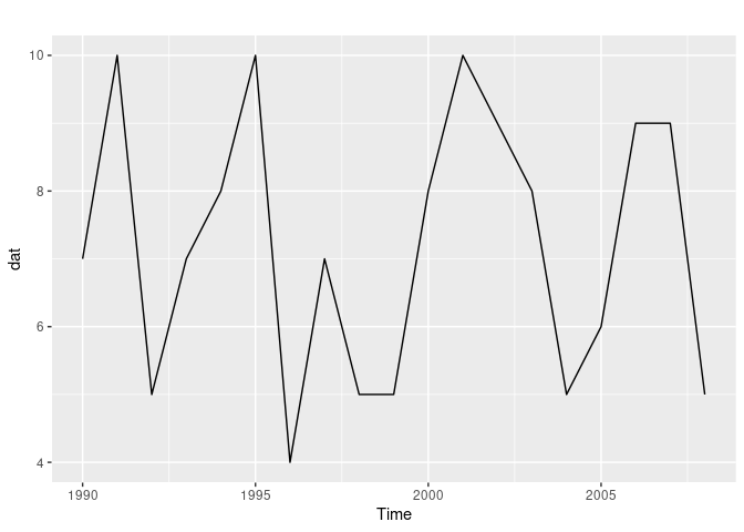
dat <- ts(dat <- c(7,10,5,7,8,10,4,7,5,5,8,10,9,8,5,6,9,9,5), start = c(1990,1), frequency = 1)
autoplot(dat)

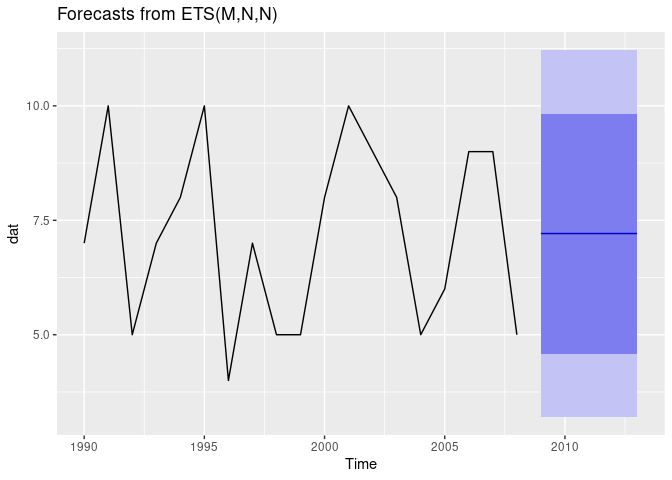
(forecast(dat, h = 5)) |> autoplot()

# intermediate
library(fpp3) # https://otexts.com/fpp3/
#> ── Attaching packages ──────────────────────────────────────────── fpp3 0.4.0 ──
#> ✔ tibble      3.1.8     ✔ tsibble     1.1.1
#> ✔ dplyr       1.0.9     ✔ tsibbledata 0.3.0
#> ✔ tidyr       1.2.0     ✔ feasts      0.2.2
#> ✔ lubridate   1.8.0     ✔ fable       0.3.1
#> ✔ ggplot2     3.3.6
#> ── Conflicts ───────────────────────────────────────────────── fpp3_conflicts ──
#> ✖ lubridate::date()      masks base::date()
#> ✖ dplyr::filter()        masks stats::filter()
#> ✖ fabletools::forecast() masks forecast::forecast()
#> ✖ tsibble::intersect()   masks base::intersect()
#> ✖ tsibble::interval()    masks lubridate::interval()
#> ✖ dplyr::lag()           masks stats::lag()
#> ✖ tsibble::setdiff()     masks base::setdiff()
#> ✖ tsibble::union()       masks base::union()
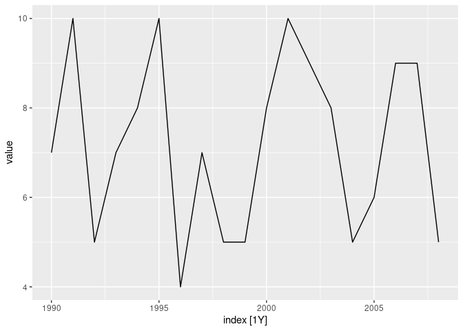
dat2 <- as_tsibble(dat)
autoplot(dat2)
#> Plot variable not specified, automatically selected `.vars = value`

ACF(dat2) |> autoplot()
#> Response variable not specified, automatically selected `var = value`

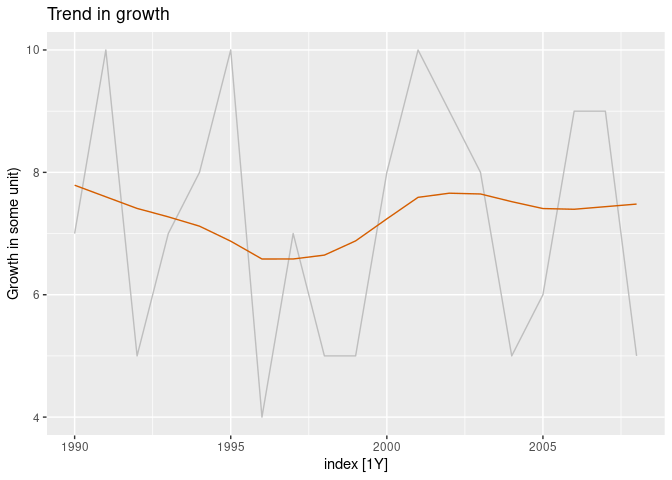
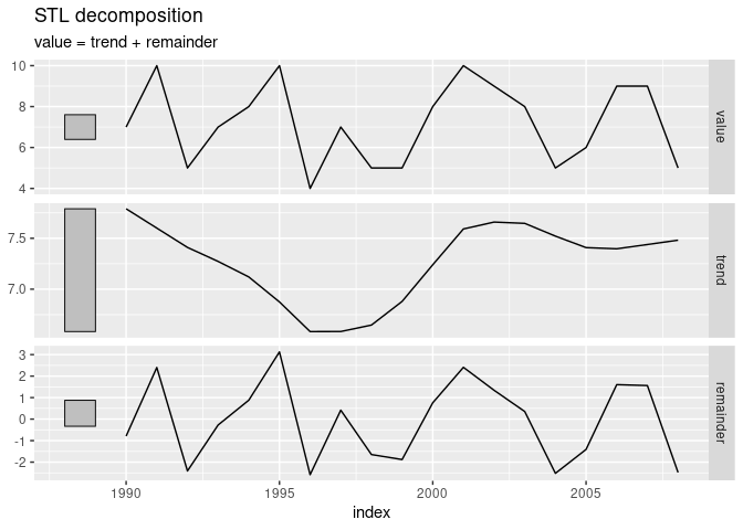
dcmp <- dat2 |> model(stl = STL(value))
components(dcmp)
#> # A dable: 19 x 6 [1Y]
#> # Key:     .model [1]
#> # :        value = trend + remainder
#>    .model index value trend remainder season_adjust
#>    <chr>  <dbl> <dbl> <dbl>     <dbl>         <dbl>
#>  1 stl     1990     7  7.79    -0.790             7
#>  2 stl     1991    10  7.6      2.4              10
#>  3 stl     1992     5  7.41    -2.41              5
#>  4 stl     1993     7  7.27    -0.273             7
#>  5 stl     1994     8  7.12     0.880             8
#>  6 stl     1995    10  6.87     3.13             10
#>  7 stl     1996     4  6.58    -2.58              4
#>  8 stl     1997     7  6.58     0.416             7
#>  9 stl     1998     5  6.65    -1.65              5
#> 10 stl     1999     5  6.88    -1.88              5
#> 11 stl     2000     8  7.24     0.76              8
#> 12 stl     2001    10  7.59     2.41             10
#> 13 stl     2002     9  7.66     1.34              9
#> 14 stl     2003     8  7.65     0.353             8
#> 15 stl     2004     5  7.52    -2.52              5
#> 16 stl     2005     6  7.41    -1.41              6
#> 17 stl     2006     9  7.40     1.60              9
#> 18 stl     2007     9  7.44     1.56              9
#> 19 stl     2008     5  7.48    -2.48              5
components(dcmp) |>
  as_tsibble() |>
  autoplot(value, colour="gray") +
  geom_line(aes(y=trend), colour = "#D55E00") +
  labs(
    y = "Growth in some unit)",
    title = "Trend in growth"
  )

components(dcmp) %>% autoplot()

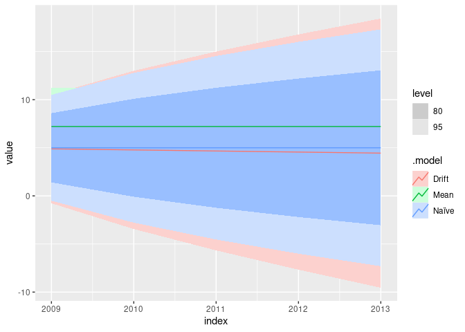
fit <- dat2 |>
  model(
    Mean = MEAN(value),
    `Naïve` = NAIVE(value),
    Drift = NAIVE(value ~ drift())
  )

fit |> forecast(h = 5) |> autoplot()

^{Created on 2022-12-06 by the reprex package (v2.0.1)}