Add Linear Discriminant Analysis Line and Show Equation on ggplot (Rstudio)

Rather than using an incorrect line generated by lm using geom_smooth(method = lm), I wanted to plot the line that a linear discriminant analysis would consider "0." I understand how to get the output data with LD1 and LD2, but not the specific equation it generates, or how to add this line to a ggplot with the X and Y values used as an input.

##Create dataframe
Size<-c(6,6,6,8,8,8,10,10,10,12,12,12,15,15,15,6,6,8,8,8,10,10,10,12,12,12,15,15,15,6,6,6,8,10,10,10,12,12,12,15,15,6,8,8,8,10,10,10,12,12,15,15)

Category<-c("ClassII", "ClassII", "ClassII", "ClassII", "ClassII", "ClassII", "ClassII", "ClassII", "ClassII", "ClassII", "ClassII", "ClassII", "ClassII", "ClassII", "ClassII", "ClassIII", "ClassIII", "ClassIII", "ClassIII", "ClassIII", "ClassIII", "ClassIII", "ClassIII", "ClassIII", "ClassIII", "ClassIII", "ClassIII", "ClassIII", "ClassIII", "ClassI", "ClassI", "ClassI", "ClassI", "ClassI", "ClassI", "ClassI", "ClassI", "ClassI", "ClassI", "ClassI", "ClassI", "ClassIV", "ClassIV", "ClassIV", "ClassIV", "ClassIV", "ClassIV", "ClassIV", "ClassIV", "ClassIV", "ClassIV", "ClassIV")

    H<-c(0.4597714,0.3384975,0.2438867,0.5773447,0.5424548,0.5225763,0.5773447,0.5424548,0.5225763,0.6188187,0.5979812,0.5321799,0.6028551,0.4706633,0.4867061,0.3674625,0.3430894,0.3102022,0.4380490,0.4037123,0.3904491,0.3952290,0.3964599,0.5618259,0.5479117,0.6004870,0.5838193,0.5983880,0.5864260,0.6313169,0.5161577,0.5822030,0.6525793,0.4346467,0.4190352,0.4248726,0.5149471,0.5433182,0.4797744,0.5149471,0.5433182,0.3071416,0.3227957,0.5113163,0.5167215,0.3055734,0.2595054,0.2697147,0.1945752,0.1844296,0.4543830,0.4506419)

    D<-c(17.060473,17.247823,17.487762,14.783000,13.305876,11.955035,15.569631,16.330392,15.297604,13.801903,13.316480,12.114558,14.744418,16.776991,14.128221,42.428042,40.711409,45.048931,44.613229,34.386670,23.555482,24.578951,22.834340,16.106533,19.230402,18.609950,25.945419,17.957438,24.540131,9.217218,8.346780,8.350304,8.931497,7.871861,7.627603,8.483040,8.952785,7.902581,4.846481,9.441160,9.461342,34.636275,33.427111,36.670034,19.104717,34.539788,44.268683,38.370184,31.623433,33.561326,45.195551,27.661643)

data<-data.frame(Size,Category,H,D)

##Creates plot I want to add LDA line and equation to
ggplot(data, aes(x=D, y=H)) + geom_point(aes(x = D, y = H, color = data$Size, shape=data$Category), size = 4) + scale_color_gradient(breaks=c(6, 8, 10, 12, 15),low = "blue1", high = "red1")+xlab("D") +ylab("H")+theme_classic()+theme(legend.position = "none")

##LDA
varsDH <- cbind(data$H, data$D)
post_hocDH <-lda(data$Category~ varsDH, CV = F)
plot_ldaDHbyCategory <- data.frame(data[, "H"], lda =predict(post_hocDH)$x)
Not sure what is meant. Same as decision boundary or discriminate line?

I believe the discriminant line--the line used to separate points above and below "0."

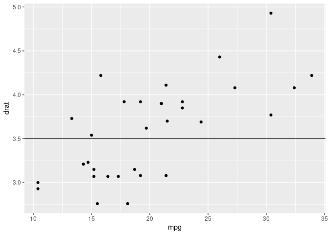
That's just

library(ggplot2)
mtcars |> ggplot(aes(mpg,drat)) +
  geom_point() +
  geom_hline(yintercept = 3.5)

Created on 2023-05-02 by the reprex package (v2.0.1)

but that may not be a discriminate line necessarily

It is possible I misunderstood. In that case, what I am looking for may indeed be the discriminate line.

Essentially, I am looking for a line that would look similar to that generated by geom_smooth(method = lm), but calculated using LDA. This line should follow the pattern of the data.

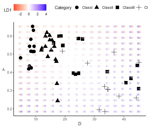
you want to see on your current plot, where LD1 and LD2 are approaching zero ?
I think the following visually represents that. its a sort of a heatmap for what ld1 and ld2 values are across the plot pane with the current axis of D and H for x and y respectively. the gradient I chose is 0 as white; for each pair of points; the left side one is LD1 and the right side one is LD2

image
the code for the above is

library(tidyverse)
##Create dataframe
Size<-c(6,6,6,8,8,8,10,10,10,12,12,12,15,15,15,6,6,8,8,8,10,10,10,12,12,12,15,15,15,6,6,6,8,10,10,10,12,12,12,15,15,6,8,8,8,10,10,10,12,12,15,15)

Category<-c("ClassII", "ClassII", "ClassII", "ClassII", "ClassII", "ClassII", "ClassII", "ClassII", "ClassII", "ClassII", "ClassII", "ClassII", "ClassII", "ClassII", "ClassII", "ClassIII", "ClassIII", "ClassIII", "ClassIII", "ClassIII", "ClassIII", "ClassIII", "ClassIII", "ClassIII", "ClassIII", "ClassIII", "ClassIII", "ClassIII", "ClassIII", "ClassI", "ClassI", "ClassI", "ClassI", "ClassI", "ClassI", "ClassI", "ClassI", "ClassI", "ClassI", "ClassI", "ClassI", "ClassIV", "ClassIV", "ClassIV", "ClassIV", "ClassIV", "ClassIV", "ClassIV", "ClassIV", "ClassIV", "ClassIV", "ClassIV")

H<-c(0.4597714,0.3384975,0.2438867,0.5773447,0.5424548,0.5225763,0.5773447,0.5424548,0.5225763,0.6188187,0.5979812,0.5321799,0.6028551,0.4706633,0.4867061,0.3674625,0.3430894,0.3102022,0.4380490,0.4037123,0.3904491,0.3952290,0.3964599,0.5618259,0.5479117,0.6004870,0.5838193,0.5983880,0.5864260,0.6313169,0.5161577,0.5822030,0.6525793,0.4346467,0.4190352,0.4248726,0.5149471,0.5433182,0.4797744,0.5149471,0.5433182,0.3071416,0.3227957,0.5113163,0.5167215,0.3055734,0.2595054,0.2697147,0.1945752,0.1844296,0.4543830,0.4506419)

D<-c(17.060473,17.247823,17.487762,14.783000,13.305876,11.955035,15.569631,16.330392,15.297604,13.801903,13.316480,12.114558,14.744418,16.776991,14.128221,42.428042,40.711409,45.048931,44.613229,34.386670,23.555482,24.578951,22.834340,16.106533,19.230402,18.609950,25.945419,17.957438,24.540131,9.217218,8.346780,8.350304,8.931497,7.871861,7.627603,8.483040,8.952785,7.902581,4.846481,9.441160,9.461342,34.636275,33.427111,36.670034,19.104717,34.539788,44.268683,38.370184,31.623433,33.561326,45.195551,27.661643)

data<-data.frame(Size,Category,H,D)
## Creates plot I want to add LDA line and equation to
(p1 <- ggplot(data) +
  geom_point(aes(x = D, y = H, size = Size, shape = Category), size = 4) +
  xlab("D") +
  ylab("H") +
  theme_classic() +
  theme(legend.position = "top"))

##LDA
library(MASS)
post_hocDH <-lda(Category~ H + D , CV = F,data = data)


nx <- 16; ny <- 16
rd <- range(data$D)
rh <- range(data$H)
xg<-seq(rd[[1]],rd[[2]],length=nx)
yg<-seq(rh[[1]],rh[[2]],length=ny)
xyg <- expand.grid(D=xg,H=yg)
ld_grid <- cbind(xyg,predict(post_hocDH,
                             newdata = xyg)$x)
p1 + geom_point(
  data = ld_grid,
  aes(
    x = D,
    y = H,
    colour = LD1
  ),
  size=2,
  alpha = 0.3,
  position = position_nudge(x = -.3)
) + geom_point(
  data = ld_grid,
  aes(
    x = D,
    y = H,
    colour = LD2
  ),
  size=2,
  alpha = 0.3,
  position = position_nudge(x = .3)
)+scale_color_gradient2(low = 'red',
                        high = 'blue')

This topic was automatically closed 42 days after the last reply. New replies are no longer allowed.

If you have a query related to it or one of the replies, start a new topic and refer back with a link.