Authors: Bill Schmid - Twitter - GitHub
View the Table - Repo
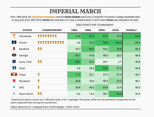
Using gt to produce table for 2020/Week 41 Tidy Tuesday on Women's College Basketball.
library(tidyverse)
library(tidytuesdayR)
library(gt)
library(paletteer)
library(showtext)

# pulling in data ---------------------------------------------------------

tidy_year <- 2020
tidy_week <- 41

tuesdata <- tt_load(tidy_year, week = tidy_week)

tournament <- tuesdata$tournament %>%
  mutate(school = as_factor(school))

# lookup table for seed points
seed_point_table <-
  tribble(
    ~seed, ~points,
    1, 	100,
    2, 	72.7,
    3, 	54.5,
    4,	48.5,
    5,	33.3,
    6,	33.3,
    7,	27.3,
    8,	21.2,
    9,	18.2,
    10,	18.2,
    11,	18.2,
    12,	15.2,
    13,	9.09,
    14,	6.06,
    15,	3.03,
    16,	0
  )

# wrangling ---------------------------------------------------------------

# dataset starts in 1982 and ends in 2018 so not quite 4 decades. Spans 37 years
sample_years <- 37

uconn_seed <- tournament %>%
  filter(school == 'UConn')

# adding in trophy emoji for first place
tournament_trophy <- tournament %>%
  mutate(champs = case_when(
    tourney_finish == "Champ" ~ "🏆",
    TRUE ~ "")) %>%
  group_by(school) %>%
  mutate(total_champs = paste0(champs, collapse = "")) %>%
  ungroup() %>%
  distinct(school, .keep_all=TRUE) %>%
  select(school, total_champs)

# seed points by decade

seed_pts <- tournament %>%
  left_join(seed_point_table, by = "seed") %>%
  mutate(decade = floor(year / 10) * 10) %>%
  group_by(school, decade) %>%
  summarise(total_decade_pts = sum(points)) %>%
  ungroup() %>%
  mutate(decade_avg = case_when(
    decade < 1990 ~ total_decade_pts / 8,
    decade > 2009 ~ total_decade_pts / 9,
    TRUE ~ total_decade_pts / 10))

# seed points top 10 overall
top_10_overall <- seed_pts %>%
  group_by(school) %>%
  summarise(total_overall = sum(total_decade_pts)) %>%
  mutate(overall = total_overall / sample_years) %>%
  slice_max(overall, n=10) %>%
  select(-total_overall)

top_10_final <- seed_pts %>%
  filter(school %in% top_10_overall$school) %>%
  select(-total_decade_pts) %>%
  pivot_wider(names_from = decade, values_from = decade_avg) %>%
  mutate(across(everything(), ~replace_na(.x, 0))) %>%
  left_join(top_10_overall, by = "school") %>%
  ungroup() %>%
  arrange(desc(overall)) %>%
  # below mutate adds in images to the dataset
  mutate(img = paste0("https://raw.githubusercontent.com/schmid07/TT-2020-Week-41/main/img/", school, ".jpg")) %>%
  left_join(tournament_trophy) %>%
  mutate(school = recode_factor(school, 'North Carolina' = 'UNC'),
         school = recode_factor(school, 'Louisiana Tech' = 'Louis. Tech')) %>%
  select(img, school, total_champs, everything())


# creating table ----------------------------------------------------------

final_table <- top_10_final %>%
  gt() %>%
  text_transform(
    locations = cells_body(vars(img)),
    fn = function(x){
      web_image(url = x, height = 20)
    }) %>%
  opt_table_font(font = google_font(name = 'Open Sans')) %>%
  cols_width(
    vars(img) ~ px(55),
    vars(school,overall) ~ (px(120)),
    vars(total_champs) ~ (px(200)),
    vars("1980", "1990", "2000", "2010") ~ px(90)
  ) %>%
  cols_align(
    columns = vars(img),
    align = "center") %>%
  cols_align(
    columns = vars('school'),
    align = "left") %>%
  data_color(
    columns=vars("1980", "1990", "2000", "2010", overall),
    colors = scales::col_numeric(
      palette = as.character(paletteer::paletteer_d("ggsci::green_material", n = 5)),
      domain = NULL)) %>%
  fmt_number(columns = vars("1980", "1990", "2000", "2010", overall),
               decimals = 1) %>%
  tab_options(table.background.color = '#f9f9f9',
              table.border.top.color = "#36454f",
              table.border.bottom.color = "#36454f") %>%
  tab_style(style=list(cell_borders(
                 sides = "left",
                 color = "black",
                 weight = px(3))),
    locations=list(
      cells_body(
        columns = vars(overall)))) %>%
  tab_style(
    style = list(cell_borders(
      sides = "bottom",
      color = "black",
      weight = px(3))),
    locations = list(
      cells_column_labels(
        columns = gt::everything()))) %>%
  tab_style(
    style = cell_text(
      font = google_font(name = 'Rye'),
      weight = 'bold',
      size = px(35),
      align = 'center'),
    locations = cells_title(groups = 'title')) %>%
  tab_style(
    style = cell_text(
      size = px(15),
      style = 'italic',
      align = 'center'),
    locations = cells_title(groups = 'subtitle')) %>%
  tab_style(
    style=cell_text(
      weight = 'bold',
      size = px(15),
      align = 'center'),
    locations = cells_column_labels(gt::everything())) %>%
  cols_label(
    img = "",
    school = "SCHOOL",
    total_champs = "CHAMPIONSHIPS",
    overall = "OVERALL",
    "1980" = "1980s",
    "1990" = "1990s",
    "2000" = "2000s",
    "2010" = "2010s") %>%
  tab_source_note("TABLE: @schmid_07 | Adapted from: FiveThirtyEight | DATA: NCAA") %>%
  tab_header(title = "IMPERIAL MARCH",
             subtitle = html("From 1982-2018, the
             <b style = 'color:#FF8200'>Tennessee Volunteers</b>
             and the
             <b style = 'color:#000E2F'>UConn Huskies </b>
             have won a combined 19 women's college basketball titles. In every year from 2007-2018,
             <b style = 'color:#000E2F'>UConn </b>
             was awarded a #1 seed, a streak broken in 2019, when
             <b style = 'color:#000E2F'>UConn </b>
             was awarded a #2 seed. <br> ")) %>%
  tab_spanner(label = "SEED POINTS PER TOURNAMENT", columns = 4:7) %>%
  tab_footnote(footnote = "Seed points award a score on a 100-point scale;
               a No.1 seed gets 100 points, while the rest descend in proportion to
               the seed's expected wins during the tournament",
    locations = cells_column_labels(columns = 8))


path <- here::here("plots",
                   glue::glue(tidy_year, "_", tidy_week, "_", ".png"))

path_2 <- here::here("plots",
                     glue::glue(tidy_year, "_", tidy_week, ".html"))

gtsave(final_table, path)
gtsave(final_table, path_2)
