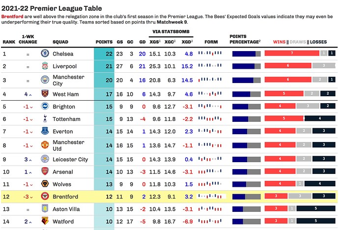
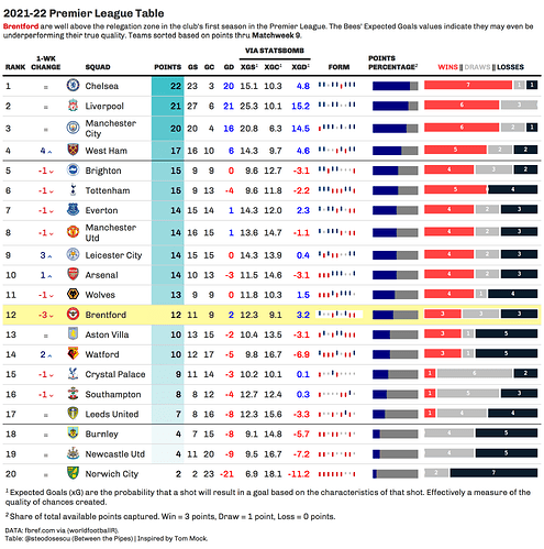
Sorry. for resurrecting an old topic. I am trying to reproduce this table, with the same data and with different data, but I always find the same problem. If you enter a certain number of matchdays (38 for example), the created dataframe (joined_df) will only recognise 32. The first dataframe (games_df) is created correctly and has 38 matchdays, if anyone is interested try running this part of the script:
library(tidyverse)
library(worldfootballR) # installed using "remotes::install_github("JaseZiv/worldfootballR")"
library(gt) # for beautiful static tables
library(gtExtras) # for add-ons working with {gt} package
library(magick)
library(webshot) # saving high quality images of gt tables
library(glue)
library(ggimage) # for working with logos
library(rlang)
library(RCurl)

##### Data import: Load data from {worldfootballR} and other sources #####

# Function to extract Premier League match results data from FBREF
EPL_2022 <- get_match_results(country = "ENG", gender = "M", season_end_year = 2022, tier = "1st")

# Load team mapping file
team_mapping <- "https://raw.githubusercontent.com/steodose/Club-Soccer-Forecasts/main/team_mapping.csv" %>%
  read_csv()

##### Set up themes for table #####

# Define color palette to use in tables
my_color_pal <- c("#ffffff", "#f2fbd2", "#c9ecb4", "#93d3ab", "#35b0ab")

# Create 538 GT table theme from Thomas Mock's blog.
gt_theme_538 <- function(data, ...) {
  data %>%
    # Add team logos w/ web_image
    text_transform(
      locations = cells_body(
        vars(url_logo_espn)
      ),
      fn = function(x) {
        web_image(
          url = x,
          height = 25
        )
      }
    ) %>%
    # Relabel columns
    cols_label(
      url_logo_espn = ""
    ) %>%
    opt_all_caps() %>%
    opt_table_font(
      font = list(
        google_font("Chivo"),
        default_fonts()
      )
    ) %>%
    tab_style(
      style = cell_borders(
        sides = "bottom", color = "transparent", weight = px(2)
      ),
      locations = cells_body(
        columns = TRUE,
        # This is a relatively sneaky way of changing the bottom border
        # Regardless of data size
        rows = nrow(data$`_data`)
      )
    ) %>%
    tab_options(
      column_labels.background.color = "white",
      table.border.top.width = px(3),
      table.border.top.color = "transparent",
      table.border.bottom.color = "transparent",
      table.border.bottom.width = px(3),
      column_labels.border.top.width = px(3),
      column_labels.border.top.color = "transparent",
      column_labels.border.bottom.width = px(3),
      column_labels.border.bottom.color = "black",
      data_row.padding = px(3),
      source_notes.font.size = 12,
      table.font.size = 16,
      heading.align = "left",
      ...
    )
}

matchweek <- 38 # Specify how many full matchweeks have been played
last_week <- matchweek - 1

games_df <- EPL_2022 %>%
  filter(Wk <= matchweek) %>%
  mutate(Result = HomeGoals - AwayGoals) %>%
  select(Home, Away, Result, Wk, HomeGoals, AwayGoals, Home_xG, Away_xG) %>%
  pivot_longer(Home:Away, names_to = "home_away", values_to = "Team") %>%
  mutate(
    Result = ifelse(home_away == "Home", Result, -Result),
    win = ifelse(Result == 0, 0.5, ifelse(Result > 0, 1, 0))
  ) %>%
  select(Wk, Team, HomeGoals, AwayGoals, win, Result) %>%
  drop_na()

team_mapping2 <- team_mapping %>%
  select(squad_fbref, url_logo_espn)

joined_df <- games_df %>%
  group_by(Team) %>%
  summarise(
    Wins = length(win[win == 1]),
    Losses = length(win[win == 0]),
    Draws = length(win[win == 0.5]),
    MP = sum(Wins, Losses, Draws),
    Points = (Wins * 3) + (Draws * 1),
    `Points Percentage` = (100 * Points / (MP * 3)),
    GD = sum(Result),
    form = list(win), .groups = "drop"
  ) %>%
  left_join(team_mapping2, by = c("Team" = "squad_fbref")) %>%
  select(url_logo_espn, Team, Points, MP, Wins, Draws, Losses, GD, `Points Percentage`, form) %>%
  arrange(desc(Points), desc(GD)) %>%
  ungroup() %>%
  mutate(Rank = row_number()) %>%
  relocate(Rank) %>%
  rename(Squad = Team) %>%
  mutate(list_data = list(c(Wins, Draws, Losses)))
By not recognising those other six games, the final table is incorrect.

