I am working on a project involving time series data with Gaussian noise, and I am encountering an issue with parameter estimation. Specifically, my estimated parameter psi differs significantly from the true value used in the data generation.
I generate Gaussian noise data using the following function in R:
simulate_data_gaussian <- function(T, a0, b0, psi0, sigma0) {
  epsilon <- rnorm(T - 1, mean = 0, sd = sigma0)
  y <- numeric(T)
  e <- numeric(T)
  e[1] <- rnorm(1, mean = 0, sd = sigma0)
  y[1] <- a0 + b0 * 1 + e[1]
  for (t in 2:T) {
    e[t] <- psi0 * e[t-1] + epsilon[t-1]
    y[t] <- a0 + b0 * t + e[t]
  }
  return(y)
}
I use this objective function to estimate parameters a, b, and psi:
f_objective <- function(a, b, psi, y, T) {
  residuals <- y[2:T] - a - b * (2:T) - psi * (y[1:(T-1)] - a - b * (1:(T-1)))
  return(sum(residuals^2) / T)
}
The complete code for the simulation is below:
# Simulated data (Gaussian)
set.seed(123)
T <- 100 # Sample size
a0 <- 1
b0 <- 2
psi0 <- 0.5
sigma0 <- 1
y <- simulate_data_gaussian(T, a0, b0, psi0, sigma0)
# Objective function f(a,b,psi)
f_objective <- function(a, b, psi, y, T) {
residuals <- y[2:T] - a - b * (2:T) - psi * (y[1:(T-1)] - a - b * (1:(T-1)))
return(sum(residuals^2) / T)
}
# Analytical solution for a and b in terms of psi
solve_ab_psi <- function(psi, y, T) {
# Construct the system of linear equations for a and b
A <- matrix(0, nrow = 2, ncol = 2)
b_vec <- numeric(2)
for (t in 2:T) {
A[1, 1] <- A[1, 1] + 1 + psi^2
A[1, 2] <- A[1, 2] + t + psi * (t - 1)
A[2, 1] <- A[2, 1] + t + psi * (t - 1)
A[2, 2] <- A[2, 2] + t^2 + (t - 1)^2
b_vec[1] <- b_vec[1] + y[t] + psi * y[t-1]
b_vec[2] <- b_vec[2] + t * y[t] + (t - 1) * psi * y[t-1]
}
# Solve for a(psi) and b(psi)
solution <- solve(A, b_vec)
a_psi <- solution[1]
b_psi <- solution[2]
return(c(a_psi, b_psi))
}
# Function to compute f(a(psi), b(psi), psi)
f_psi <- function(psi, y, T) {
ab <- solve_ab_psi(psi, y, T)
a_psi <- ab[1]
b_psi <- ab[2]
return(f_objective(a_psi, b_psi, psi, y, T))
}
# Generate psi values and evaluate f(psi)
psi_values <- seq(-1, 1, by = 0.01)
f_values <- sapply(psi_values, f_psi, y = y, T = T)
# Plot f(psi)
library(ggplot2)
df <- data.frame(psi = psi_values, f_value = f_values)
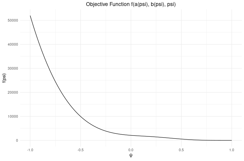
ggplot(df, aes(x = psi, y = f_value)) +
geom_line() +
labs(title = "Objective Function f(a(psi), b(psi), psi)",
x = expression(psi), y = "f(psi)") +
theme_minimal() +
theme(plot.title = element_text(hjust = 0.5))
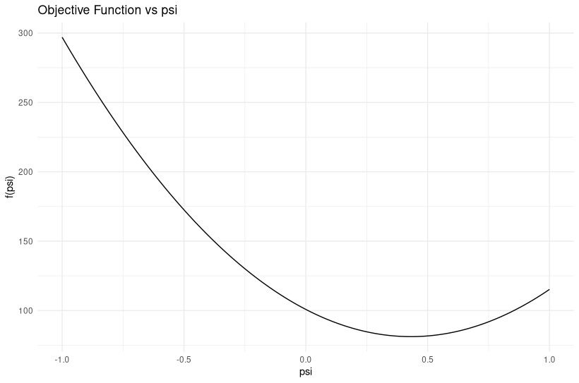
And the resulting estimations are shown in the figure below:
Issue: Despite generating data with psi0=0.5, my estimated psi is significantly different from 0.5 (0.98). I validated the generated data and objective function, but the discrepancy persists.
Question: Can someone help me understand why the estimated psi is different from the true value psi0? What might be going wrong in my estimation process?