See the FAQ: How to do a minimal reproducible example reprex for beginners. It's not difficult to convert the table to a data frame but the unnecessary effort is an impediment to receiving answers.
The following example has been derived from [this post]((ANOVA in R - Stats and R) using your data and should be studied using that link.
suppressPackageStartupMessages({
library(car)
library(dplyr)
library(ggplot2)
library(ggpubr)
library(multcomp)
library(palmerpenguins)
library(patchwork)
})
dat <- data.frame(
Parent =
as.factor(c("Mock", "Mock", "Mock", "Mock", "Mock", "Mock", "Mock", "Mock", "Mock", "Mock", "Mock", "Mock", "Mock", "Mock", "Mock", "Mock", "Mock", "Mock", "Mock", "Mock", "Mock", "Mock", "Mock", "Mock", "Mock", "Mock", "Mock", "Mock", "Mock", "Mock", "Mock", "Mock", "Mock", "Mock", "Mock", "Mock", "Mock", "Mock", "Mock", "Mock", "Mock", "Mock", "Pst_I", "Pst_I", "Pst_I", "Pst_I", "Pst_I", "Pst_I", "Pst_I", "Pst_I", "Pst_I", "Pst_I", "Pst_I", "Pst_I", "Pst_I", "Pst_I", "Pst_I", "Pst_I", "Pst_I", "Pst_I", "Pst_I", "Pst_I", "Pst_I", "Pst_I", "Pst_I", "Pst_I", "Pst_I", "Pst_I", "Pst_I", "Pst_I", "Pst_I", "Pst_I", "Pst_I", "Pst_I", "Pst_I", "Pst_I", "Pst_I", "Pst_I", "Pst_I", "Pst_I", "Pst_I", "Pst_I", "Pst_I", "Pst_I", "Pst_II", "Pst_II", "Pst_II", "Pst_II", "Pst_II", "Pst_II", "Pst_II", "Pst_II", "Pst_II", "Pst_II", "Pst_II", "Pst_II", "Pst_II", "Pst_II", "Pst_II", "Pst_II", "Pst_II", "Pst_II", "Pst_II", "Pst_II", "Pst_II", "Pst_II", "Pst_II", "Pst_II", "Pst_II", "Pst_II", "Pst_II", "Pst_II", "Pst_II", "Pst_II", "Pst_II", "Pst_II", "Pst_II", "Pst_II", "Pst_II", "Pst_II", "Pst_II", "Pst_II", "Pst_II", "Pst_II", "Pst_II", "Pst_II", "Pst_III", "Pst_III", "Pst_III", "Pst_III", "Pst_III", "Pst_III", "Pst_III", "Pst_III", "Pst_III", "Pst_III", "Pst_III", "Pst_III", "Pst_III", "Pst_III", "Pst_III", "Pst_III", "Pst_III", "Pst_III", "Pst_III", "Pst_III", "Pst_III", "Pst_III", "Pst_III", "Pst_III", "Pst_III", "Pst_III", "Pst_III", "Pst_III", "Pst_III", "Pst_III", "Pst_III", "Pst_III", "Pst_III", "Pst_III", "Pst_III", "Pst_III", "Pst_III", "Pst_III", "Pst_III", "Pst_III", "Pst_III", "Pst_III")),
Line =
as.factor(c("M1", "M1", "M1", "M1", "M1", "M1", "M1", "M1", "M1", "M1", "M1", "M2", "M2", "M2", "M2", "M2", "M2", "M2", "M2", "M3", "M3", "M3", "M3", "M3", "M3", "M3", "M3", "M3", "M3", "M3", "M3", "M3", "M4", "M4", "M4", "M4", "M4", "M4", "M4", "M4", "M4", "M4", "Pst_I_1", "Pst_I_1", "Pst_I_1", "Pst_I_1", "Pst_I_1", "Pst_I_1", "Pst_I_1", "Pst_I_1", "Pst_I_1", "Pst_I_1", "Pst_I_1", "Pst_I_2", "Pst_I_2", "Pst_I_2", "Pst_I_2", "Pst_I_2", "Pst_I_2", "Pst_I_2", "Pst_I_2", "Pst_I_2", "Pst_I_2", "Pst_I_2", "Pst_I_3", "Pst_I_3", "Pst_I_3", "Pst_I_3", "Pst_I_3", "Pst_I_3", "Pst_I_3", "Pst_I_3", "Pst_I_3", "Pst_I_3", "Pst_I_4", "Pst_I_4", "Pst_I_4", "Pst_I_4", "Pst_I_4", "Pst_I_4", "Pst_I_4", "Pst_I_4", "Pst_I_4", "Pst_I_4", "Pst_II_1", "Pst_II_1", "Pst_II_1", "Pst_II_1", "Pst_II_1", "Pst_II_1", "Pst_II_1", "Pst_II_1", "Pst_II_1", "Pst_II_1", "Pst_II_1", "Pst_II_2", "Pst_II_2", "Pst_II_2", "Pst_II_2", "Pst_II_2", "Pst_II_2", "Pst_II_2", "Pst_II_2", "Pst_II_2", "Pst_II_2", "Pst_II_2", "Pst_II_3", "Pst_II_3", "Pst_II_3", "Pst_II_3", "Pst_II_3", "Pst_II_3", "Pst_II_3", "Pst_II_3", "Pst_II_3", "Pst_II_3", "Pst_II_4", "Pst_II_4", "Pst_II_4", "Pst_II_4", "Pst_II_4", "Pst_II_4", "Pst_II_4", "Pst_II_4", "Pst_II_4", "Pst_II_4", "Pst_III_1", "Pst_III_1", "Pst_III_1", "Pst_III_1", "Pst_III_1", "Pst_III_1", "Pst_III_1", "Pst_III_1", "Pst_III_1", "Pst_III_1", "Pst_III_1", "Pst_III_2", "Pst_III_2", "Pst_III_2", "Pst_III_2", "Pst_III_2", "Pst_III_2", "Pst_III_2", "Pst_III_2", "Pst_III_2", "Pst_III_2", "Pst_III_2", "Pst_III_3", "Pst_III_3", "Pst_III_3", "Pst_III_3", "Pst_III_3", "Pst_III_3", "Pst_III_3", "Pst_III_3", "Pst_III_3", "Pst_III_3", "Pst_III_4", "Pst_III_4", "Pst_III_4", "Pst_III_4", "Pst_III_4", "Pst_III_4", "Pst_III_4", "Pst_III_4", "Pst_III_4", "Pst_III_4")),
Log =
c(8.055155783, 6.173051289, 6.838547899, 7.051532265, 6.890318194, 6.341863188, 5.959270051, 6.815049617, 6.082606218, 6.864741933, 6.795590584, 7.984846313, 6.250502269, 6.401850846, 7.043015595, 6.494560588, 6.714226935, 6.792170872, 6.795590584, 5.599318096, 7.43209122, 6.795590584, 7.211245462, 7.969408029, 6.507725058, 5.693530593, 6.670651848, 6.850727571, 6.781576222, 6.733121216, 5.909212475, 6.099987271, 5.730938813, 7.864741933, 6.930274078, 6.480546227, 6.83574596, 6.193530593, 6.221983018, 7.030731499, 6.225759587, 6.369621852, 7.773276591, 6.670651848, 6.409212475, 7.43209122, 5.617316922, 5.082606218, 5.983422391, 5.693530593, 6.255456413, 4.554847554, 6.933893282, 4.35587755, 4.724256832, 7.556180064, 6.723879513, 5.642893184, 5.714226935, 6.189143631, 6.821166845, 5.714226935, 5.795047036, 6.933893282, 6.901017267, 7.834331315, 5.316286927, 6.631061225, 5.253817558, 6.746285685, 5.971681843, 6.631061225, 7.403095247, 7.005155238, 6.532334069, 5.505155238, 5.082606218, 6.522536291, 6.582606218, 5.567624606, 6.381819071, 7.568591856, 5.99779361, 4.573741835, 7.706695062, 7.001242569, 3.209275221, 5.011272466, 6.155670236, 6.43209122, 5.218139604, 6.067624606, 5.306185234, 5.847064568, 3.161078569, 4.76783192, 5.779832058, 5.247135578, 6.145075586, 5.645075586, 6.741985599, 6.145075586, 6.821166845, 7.179516231, 6.583328838, 5.535953274, 7.178936398, 4.806185234, 5.272711839, 7.014019622, 5.722743605, 4.904332556, 6.93209122, 5.909212475, 7.679516231, 6.917109608, 6.02013685, 3.058760223, 6.284452387, 6.214226935, 6.182392395, 3.698680571, 6.155670236, 6.051532265, 6.218139604, 5.816779883, 7.182392395, 7.05257374, 4.757730227, 5.952787563, 6.155670236, 5.905971411, 6.52013685, 6.821166845, 5.883636214, 5.903673535, 4.573741835, 5.118301719, 4.503411074, 5.645075586, 6.838547899, 6.043015595, 2.758967537, 5.559727473, 5.901017267, 5.766594611, 5.6269695, 6.272711839, 6.210242471, 6.034151212, 2.786726201, 6.255456413, 3.068861916, 6.184666209, 6.353603736, 4.59662058, 6.903095247, 5.335181207, 6.682849067, 7.599987271, 5.743715865, 6.582606218, 5.561330043, 5.645075586, 6.480546227, 3.640511289, 6.608182479, 5.816779883))
# use only one parent line, to simplify illustration
# mocks <- dat[which(dat[,1] == "Mock"),]
summary(dat)
#> Parent Line Log
#> Mock :42 M3 : 13 Min. :2.759
#> Pst_I :42 M1 : 11 1st Qu.:5.681
#> Pst_II :42 Pst_I_1 : 11 Median :6.212
#> Pst_III:42 Pst_I_2 : 11 Mean :6.117
#> Pst_II_1: 11 3rd Qu.:6.800
#> Pst_II_2: 11 Max. :8.055
#> (Other) :100
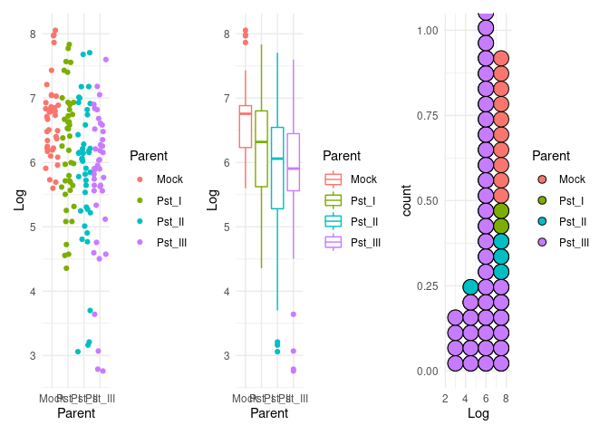
p1 <- ggplot(dat) +
aes(x = Parent, y = Log, color = Parent) +
geom_jitter() +
theme(legend.position = "none") +
theme_minimal()
p2 <- ggplot(dat) +
aes(x = Parent, y = Log, color = Parent) +
geom_boxplot() +
theme(legend.position = "none") +
theme_minimal()
p3 <- ggplot(dat) +
aes(Log, fill = Parent) +
geom_dotplot(method = "histodot", binwidth = 1.5) +
theme(legend.position = "none") +
theme_minimal()
p1 + p2 + p3
res_aov <- aov(Log ~ Parent, data = dat)

resids <- data.frame(.resid = res_aov$residuals)

# histogram
p4 <- ggplot(resids, aes(.resid)) +
  geom_histogram(color = "black", fill = "grey") +
  theme_minimal()

p5 <- ggplot(resids, aes(sample = .resid)) +
  stat_qq() +
  stat_qq_line() +
  theme_minimal()

p4 + p5
#> `stat_bin()` using `bins = 30`. Pick better value with `binwidth`.
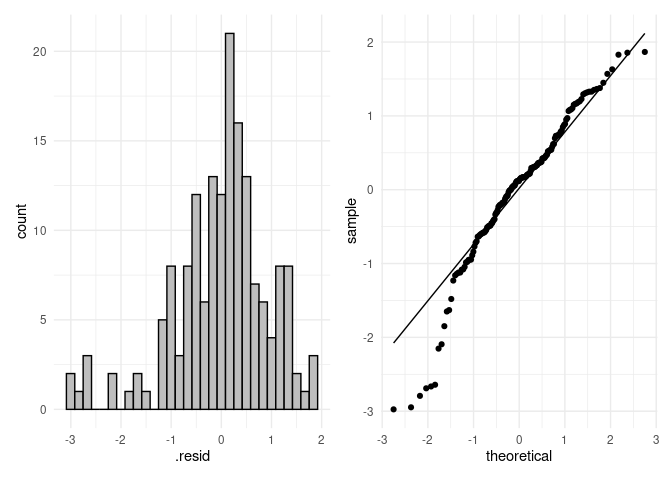
shapiro.test(res_aov$residuals)
#>
#> Shapiro-Wilk normality test
#>
#> data: res_aov$residuals
#> W = 0.95189, p-value = 1.663e-05
leveneTest(Log ~ Parent, data = dat)
#> Levene's Test for Homogeneity of Variance (center = median)
#> Df F value Pr(>F)
#> group 3 2.6809 0.04866 *
#> 164
#> ---
#> Signif. codes: 0 '***' 0.001 '**' 0.01 '*' 0.05 '.' 0.1 ' ' 1
aggregate(Log ~ Parent,
data = dat,
function(x) round(c(mean = mean(x), sd = sd(x)), 2)
)
#> Parent Log.mean Log.sd
#> 1 Mock 6.68 0.60
#> 2 Pst_I 6.20 0.91
#> 3 Pst_II 5.85 1.12
#> 4 Pst_III 5.73 1.12
group_by(dat, Parent) %>%
summarise(
mean = mean(Log, na.rm = TRUE),
sd = sd(Log, na.rm = TRUE)
)
#> # A tibble: 4 x 3
#> Parent mean sd
#> <fct> <dbl> <dbl>
#> 1 Mock 6.68 0.596
#> 2 Pst_I 6.20 0.907
#> 3 Pst_II 5.85 1.12
#> 4 Pst_III 5.73 1.12
oneway.test(Log ~ Parent,
data = dat,
var.equal = TRUE # assuming equal variances
)
#>
#> One-way analysis of means
#>
#> data: Log and Parent
#> F = 8.2319, num df = 3, denom df = 164, p-value = 3.899e-05
res_aov <- aov(Log ~ Parent,
data = dat
)
summary(res_aov)
#> Df Sum Sq Mean Sq F value Pr(>F)
#> Parent 3 22.67 7.558 8.232 3.9e-05 ***
#> Residuals 164 150.57 0.918
#> ---
#> Signif. codes: 0 '***' 0.001 '**' 0.01 '*' 0.05 '.' 0.1 ' ' 1
oneway.test(Log ~ Parent,
data = dat,
var.equal = FALSE # assuming unequal variances
)
#>
#> One-way analysis of means (not assuming equal variances)
#>
#> data: Log and Parent
#> F = 11.43, num df = 3.00, denom df = 87.72, p-value = 2.13e-06
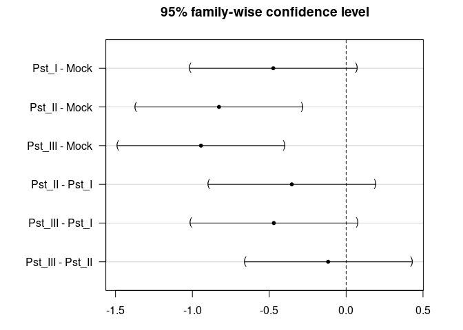
post_test <- glht(res_aov,
linfct = mcp(Parent = "Tukey")
)
summary(post_test)
#>
#> Simultaneous Tests for General Linear Hypotheses
#>
#> Multiple Comparisons of Means: Tukey Contrasts
#>
#>
#> Fit: aov(formula = Log ~ Parent, data = dat)
#>
#> Linear Hypotheses:
#> Estimate Std. Error t value Pr(>|t|)
#> Pst_I - Mock == 0 -0.4737 0.2091 -2.266 0.110
#> Pst_II - Mock == 0 -0.8271 0.2091 -3.956 <0.001 ***
#> Pst_III - Mock == 0 -0.9440 0.2091 -4.515 <0.001 ***
#> Pst_II - Pst_I == 0 -0.3533 0.2091 -1.690 0.332
#> Pst_III - Pst_I == 0 -0.4703 0.2091 -2.249 0.115
#> Pst_III - Pst_II == 0 -0.1170 0.2091 -0.559 0.944
#> ---
#> Signif. codes: 0 '***' 0.001 '**' 0.01 '*' 0.05 '.' 0.1 ' ' 1
#> (Adjusted p values reported -- single-step method)
par(mar = c(3, 8, 3, 3))
plot(post_test)

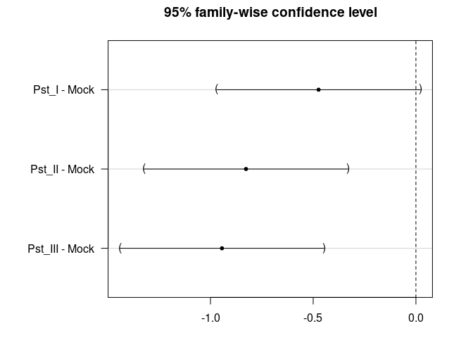
TukeyHSD(res_aov)
#>   Tukey multiple comparisons of means
#>     95% family-wise confidence level
#>
#> Fit: aov(formula = Log ~ Parent, data = dat)
#>
#> $Parent
#>                      diff        lwr         upr     p adj
#> Pst_I-Mock     -0.4737345 -1.0164396  0.06897055 0.1104074
#> Pst_II-Mock    -0.8270620 -1.3697671 -0.28435691 0.0006507
#> Pst_III-Mock   -0.9440129 -1.4867179 -0.40130778 0.0000707
#> Pst_II-Pst_I   -0.3533275 -0.8960325  0.18937762 0.3323298
#> Pst_III-Pst_I  -0.4702783 -1.0129834  0.07242675 0.1145360
#> Pst_III-Pst_II -0.1169509 -0.6596560  0.42575421 0.9438792

plot(TukeyHSD(res_aov))

# Dunnett's test:
post_test <- glht(res_aov,
                  linfct = mcp(species = "Dunnett")
)
#> Error in mcp2matrix(model, linfct = linfct): Variable(s) 'species' have been specified in 'linfct' but cannot be found in 'model'!

summary(post_test)
#>
#>   Simultaneous Tests for General Linear Hypotheses
#>
#> Multiple Comparisons of Means: Tukey Contrasts
#>
#>
#> Fit: aov(formula = Log ~ Parent, data = dat)
#>
#> Linear Hypotheses:
#>                       Estimate Std. Error t value Pr(>|t|)
#> Pst_I - Mock == 0      -0.4737     0.2091  -2.266    0.110
#> Pst_II - Mock == 0     -0.8271     0.2091  -3.956   <0.001 ***
#> Pst_III - Mock == 0    -0.9440     0.2091  -4.515   <0.001 ***
#> Pst_II - Pst_I == 0    -0.3533     0.2091  -1.690    0.332
#> Pst_III - Pst_I == 0   -0.4703     0.2091  -2.249    0.115
#> Pst_III - Pst_II == 0  -0.1170     0.2091  -0.559    0.944
#> ---
#> Signif. codes:  0 '***' 0.001 '**' 0.01 '*' 0.05 '.' 0.1 ' ' 1
#> (Adjusted p values reported -- single-step method)

par(mar = c(3, 8, 3, 3))
plot(post_test)
dat$Parent <- relevel(dat$Parent, ref = "Mock")

res_aov2 <- aov(Log ~ Parent,
                data = dat
)

# Dunnett's test:
post_test <- glht(res_aov2,
                  linfct = mcp(Parent = "Dunnett")
)

summary(post_test)
#>
#>   Simultaneous Tests for General Linear Hypotheses
#>
#> Multiple Comparisons of Means: Dunnett Contrasts
#>
#>
#> Fit: aov(formula = Log ~ Parent, data = dat)
#>
#> Linear Hypotheses:
#>                     Estimate Std. Error t value Pr(>|t|)
#> Pst_I - Mock == 0    -0.4737     0.2091  -2.266   0.0647 .
#> Pst_II - Mock == 0   -0.8271     0.2091  -3.956   <0.001 ***
#> Pst_III - Mock == 0  -0.9440     0.2091  -4.515   <0.001 ***
#> ---
#> Signif. codes:  0 '***' 0.001 '**' 0.01 '*' 0.05 '.' 0.1 ' ' 1
#> (Adjusted p values reported -- single-step method)

par(mar = c(3, 8, 3, 3))
plot(post_test)
pairwise.t.test(dat$Log, dat$Parent,
p.adjust.method = "holm"
)
#>
#> Pairwise comparisons using t tests with pooled SD
#>
#> data: dat$Log and dat$Parent
#>
#> Mock Pst_I Pst_II
#> Pst_I 0.09911 - -
#> Pst_II 0.00057 0.18592 -
#> Pst_III 7.2e-05 0.09911 0.57670
#>
#> P value adjustment method: holm
x <- which(names(dat) == "Parent") # name of grouping variable
y <- which(
names(dat) == "Log" # names of variables to test
)
method1 <- "anova" # one of "anova" or "kruskal.test"
method2 <- "t.test" # one of "wilcox.test" or "t.test"
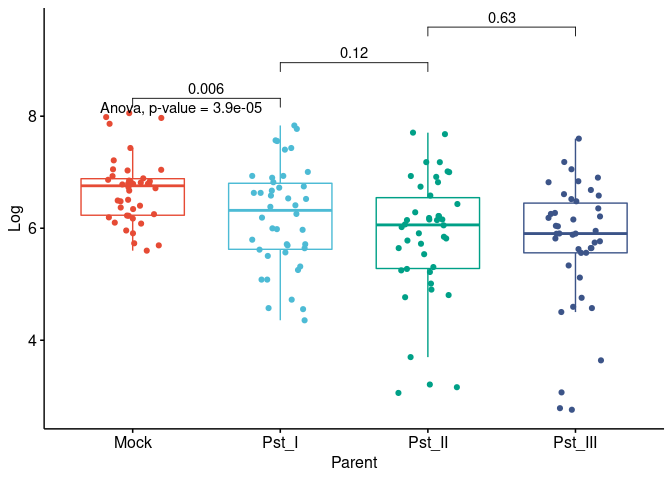
my_comparisons <- list(c("Mock", "Pst_I"), c("Pst_I", "Pst_II"), c("Pst_II", "Pst_III")) # comparisons for post-hoc tests
for (i in y) {
for (j in x) {
p <- ggboxplot(dat,
x = colnames(dat[j]), y = colnames(dat[i]),
color = colnames(dat[j]),
legend = "none",
palette = "npg",
add = "jitter"
)
print(
p + stat_compare_means(aes(label = paste0(..method.., ", p-value = ", ..p.format..)),
method = method1, label.y = max(dat[, i], na.rm = TRUE)
)
+ stat_compare_means(comparisons = my_comparisons, method = method2, label = "p.format") # remove if p-value of ANOVA or Kruskal-Wallis test >= alpha
)
}
}