Hi, and welcome!
Two preliminaries: FAQs you should review for future reference: the homework policy and how to create reproducible example, called a reprex, which really helps to pinpoint your problem.
You'll find that data analysis has three steps: 1) cleaning the data, 2) visualizing it and 3) analyzing it. I'll illustrate with an example from a data set in the dslabs package that accompanies Raphael Irizarry's text from his HarvardX course on data science.
library(dslabs)
library(dplyr)
#>
#> Attaching package: 'dplyr'
#> The following objects are masked from 'package:stats':
#>
#>     filter, lag
#> The following objects are masked from 'package:base':
#>
#>     intersect, setdiff, setequal, union
library(ggplot2)


data(heights)
summary(heights)
#>      sex          height
#>  Female:238   Min.   :50.00
#>  Male  :812   1st Qu.:66.00
#>               Median :68.50
#>               Mean   :68.32
#>               3rd Qu.:71.00
#>               Max.   :82.68
p <- ggplot(heights, aes(height))
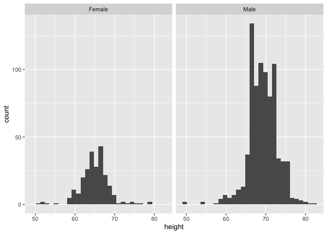
p + geom_histogram() + facet_wrap(heights$sex)
#> `stat_bin()` using `bins = 30`. Pick better value with `binwidth`.

males <- heights %>% filter(sex == "Male") %>% select(height)
summary(males)
#>      height
#>  Min.   :50.00
#>  1st Qu.:67.00
#>  Median :69.00
#>  Mean   :69.31
#>  3rd Qu.:72.00
#>  Max.   :82.68
females <- heights %>% filter(sex == "Female") %>% select(height)
summary(females)
#>      height
#>  Min.   :51.00
#>  1st Qu.:63.00
#>  Median :64.98
#>  Mean   :64.94
#>  3rd Qu.:67.00
#>  Max.   :79.00
shapiro.test(males$height)
#>
#>  Shapiro-Wilk normality test
#>
#> data:  males$height
#> W = 0.96374, p-value = 2.623e-13
shapiro.test(females$height)
#>
#>  Shapiro-Wilk normality test
#>
#> data:  females$height
#> W = 0.94255, p-value = 4.671e-08
Created on 2020-01-03 by the reprex package (v0.3.0)
The eye jumps immediately to the two histograms. Same or different populations? Well, they look kind of different. How about the summaries? How do the means, medians and quartiles differ?
What other statistical measures can we apply. You've identified one and above it is run for the population and by sex separately. To interpret each, you have to choose a null hypothesis, conventionally called H_0, an alternative hypothesis, conventionally called H_1 and a level of significance, conventionally designated as \alpha.
For the shapiro test $H_0is that the population sample is from a population with anormal distributionand, of course$H_1` is that they are not.
A common significance level is \alpha = 0.05, meaning that there is only a 1 in 20 chance of observing the test statistic if H_0 is false. I call this the laugh test. In the shapiro.test, the combined population and each subpopulation all have very small p-values leading us to fail to reject H_0. Notice that statistical tests don't prove, they simply provide evidence to a stated degree whether it is justified to accept one or the other hypotheses.
At this point, we don't have any statistical test of the differences between the two populations. We have some measures of central tendency that suggest differences, but the conclusion that both are normally distributed doesn't lead us to think that there is no difference.
Take a look at t.test and see how you can adopt it to the heights data and then to yours.