Thanks, everyone, for attempting reprexes, and welcome to RStudio Community!
Now, to fix the code!
First, a few of you missed an important detail: you didn't load ggplot2, so the error you got was about how R couldn't find that function. Remember, reprex runs R in a completely fresh session, so even if you've loaded a package in RStudio, it won't be available unless you include library() in your reprex code.
Technically, we could also make this example more minimal. The problem is not actually with the diabetes dataset, so we could use a built-in dataset to show the problem. However, our example is still reproducible (since the data is on GitHub and the code does read it correctly). Since you may not be sure if it's the data or code that's the problem, it's reasonable to include that dataset.
It turns out that the real issue is a quirk of base R. read.csv() returns a regular data frame, and when we try to subset a single column in a data frame, R converts the object to a vector, not a dataframe:
x <- data.frame(a = 1:5)

x
#>   a
#> 1 1
#> 2 2
#> 3 3
#> 4 4
#> 5 5

x[, "a"]
#> [1] 1 2 3 4 5

is.data.frame(x[, "a"])
#> [1] FALSE
ggplot() expects a data frame, not a vector. When you're dealing with base R, the solution is to set drop = FALSE, which keeps x as a data frame.
x[, "a", drop = FALSE]
#>   a
#> 1 1
#> 2 2
#> 3 3
#> 4 4
#> 5 5

is.data.frame(x[, "a", drop = FALSE])
#> [1] TRUE
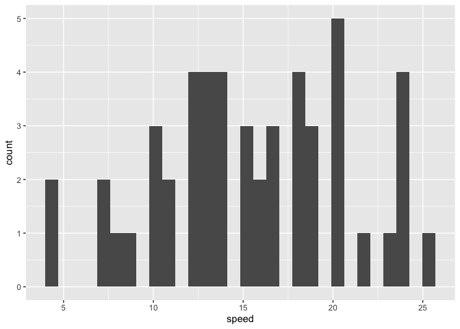
Using this approach will fix our issue. I don't actually need the diabetes dataset here, so instead, I'll use the built-in cars dataset and make a histogram of the speed variable.
library(ggplot2)
just_speed <- cars[, "speed", drop = FALSE]
ggplot(just_speed, aes(x = speed)) +
  geom_histogram()
#> `stat_bin()` using `bins = 30`. Pick better value with `binwidth`.

Notably, the original code used read.csv(), which returns a regular data frame, but readr::read_csv() returns a tibble, a special case of the data frame. Tibbles don't have this behavior, and subsetting them always returns a tibble. We don't need drop = FALSE:
library(tidyverse)
y <- tibble(a = 1:5)
y[, "a"]
#> # A tibble: 5 x 1
#>       a
#>   <int>
#> 1     1
#> 2     2
#> 3     3
#> 4     4
#> 5     5
Using a tibble also solves our problem:
library(tidyverse)
cars <- as_tibble(cars)
just_speed <- cars[, "speed"]
ggplot(just_speed, aes(x = speed)) +
  geom_histogram()
#> `stat_bin()` using `bins = 30`. Pick better value with `binwidth`.

