@loiacj, questions are absolutely the hardest part of data analysis.
There's a more direct way to get principal components than from the output of a pcr model,
PCs <- prcomp(~ Sepal.Length + Sepal.Width + Petal.Length + Petal.Width, data = iris, scale = TRUE)
PCs
#> Standard deviations (1, .., p=4):
#> [1] 1.7083611 0.9560494 0.3830886 0.1439265
#>
#> Rotation (n x k) = (4 x 4):
#> PC1 PC2 PC3 PC4
#> Sepal.Length 0.5210659 -0.37741762 0.7195664 0.2612863
#> Sepal.Width -0.2693474 -0.92329566 -0.2443818 -0.1235096
#> Petal.Length 0.5804131 -0.02449161 -0.1421264 -0.8014492
#> Petal.Width 0.5648565 -0.06694199 -0.6342727 0.5235971
summary(PCs)
#> Importance of components:
#> PC1 PC2 PC3 PC4
#> Standard deviation 1.7084 0.9560 0.38309 0.14393
#> Proportion of Variance 0.7296 0.2285 0.03669 0.00518
#> Cumulative Proportion 0.7296 0.9581 0.99482 1.00000
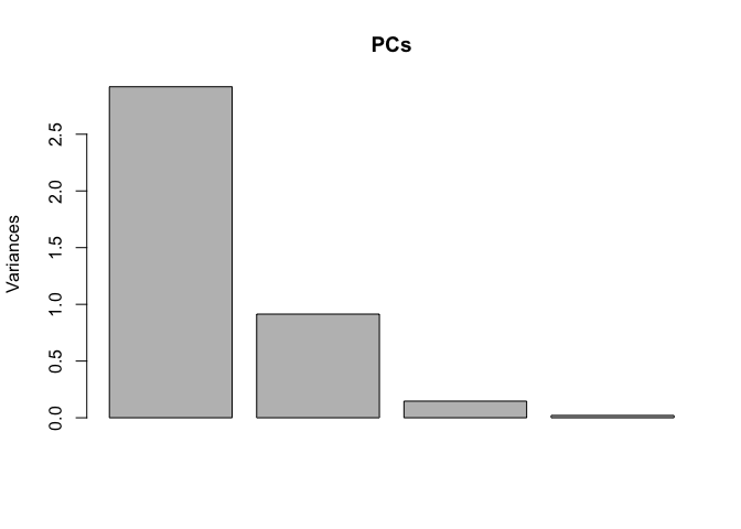
plot(PCs)
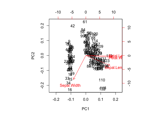
biplot(PCs)
Created on 2020-01-10 by the reprex package (v0.3.0)
The first plot demonstrates how principal components differ in their variance. The second is worth pausing over. It's a plot of all the iris data of the first (PC1) against the second (PC2) component showing vectors of the of the variables projected. This is key to understanding principal components--they are orthogonal. So, now we've gone from 2-space to n-space.
So, how to use principal components in a linear regression model? The only left-over variable, species, is categorical, and that would push us over to glm methods. So let's rerun and reserve Sepal.Length as the dependent variable.
PCs <- prcomp(~ Sepal.Width + Petal.Length + Petal.Width, data = iris, scale = TRUE)
y <- iris$Sepal.Width
fit <- lm(y~PCs$x[,1]+PCs$x[,2])
summary(fit)
#>
#> Call:
#> lm(formula = y ~ PCs$x[, 1] + PCs$x[, 2])
#>
#> Residuals:
#>        Min         1Q     Median         3Q        Max
#> -0.0139056 -0.0026317  0.0000775  0.0025267  0.0121509
#>
#> Coefficients:
#>               Estimate Std. Error t value Pr(>|t|)
#> (Intercept)  3.0573333  0.0003664  8345.3   <2e-16 ***
#> PCs$x[, 1]  -0.1822434  0.0002466  -739.0   <2e-16 ***
#> PCs$x[, 2]  -0.3952146  0.0004262  -927.3   <2e-16 ***
#> ---
#> Signif. codes:  0 '***' 0.001 '**' 0.01 '*' 0.05 '.' 0.1 ' ' 1
#>
#> Residual standard error: 0.004487 on 147 degrees of freedom
#> Multiple R-squared:  0.9999, Adjusted R-squared:  0.9999
#> F-statistic: 7.029e+05 on 2 and 147 DF,  p-value: < 2.2e-16
Created on 2020-01-10 by the reprex package (v0.3.0)
Does this point you in the right direction?