Hi, and welcome!
A reproducible example, called a reprex is needed to provide a more useful answer. Without knowing the data that the function operates on, possible problems aren't detectable.
However, that may not be possible in this case. The DCchoice package is at version 0.0.15, relies on the version package that has an archived dependency on Icens, which can be installed via BiocManager::install("Icens") after installing BiocManager. If that weren't enough, the help(dbchoice) example requires installing the Ecdat package.
After those obstacles, considerable tinkering is required to produce a reprex from the example
library(DCchoice)
#> Loading required package: MASS
#> Loading required package: interval
#> Loading required package: survival
#> Loading required package: perm
#> Loading required package: Icens
#> Loading required package: MLEcens
#> Loading required package: Formula
require("Ecdat")
#> Loading required package: Ecdat
#> Loading required package: Ecfun
#>
#> Attaching package: 'Ecfun'
#> The following object is masked from 'package:base':
#>
#>     sign
#>
#> Attaching package: 'Ecdat'
#> The following object is masked from 'package:MASS':
#>
#>     SP500
#> The following object is masked from 'package:datasets':
#>
#>     Orange
# may be necessary to install missing dependency of `intervals` dependency
# with BiocManager::install("Icens")
## Examples are based on a data set NaturalPark in the package
## Ecdat (Croissant 2011): DBDCCV style question for measuring
## willingness to pay for the preservation of the Alentejo Natural
## Park. The data set (dataframe) contains seven variables:
## bid1 (bid in the initial question), bidh (higher bid in the follow-up
## question), bidl (lower bid in the follow-up question), answers
## (response outcomes in a factor format with four levels of "nn",
## "ny", "yn", "yy"), respondents' characteristic variables such
## as age, sex and income (see NaturalPark for details).
data(NaturalPark, package = "Ecdat")
head(NaturalPark)
#>   bid1 bidh bidl answers age    sex income
#> 1    6   18    3      yy   1 female      2
#> 2   48  120   24      yn   2   male      1
#> 3   48  120   24      yn   2 female      3
#> 4   24   48   12      nn   5 female      1
#> 5   24   48   12      ny   6 female      2
#> 6   12   24    6      nn   4   male      2
## The variable answers are converted into a format that is suitable for the
## function dbchoice() as follows:
NaturalPark$R1 <- ifelse(substr(NaturalPark$answers, 1, 1) == "y", 1, 0)
NaturalPark$R2 <- ifelse(substr(NaturalPark$answers, 2, 2) == "y", 1, 0)

## We assume that the error distribution in the model is a
## log-logistic; therefore, the bid variables bid1 is converted
## into LBD1 as follows:
NaturalPark$LBD1 <- log(NaturalPark$bid1)

## Further, the variables bidh and bidl are integrated into one
## variable (bid2) and the variable is converted into LBD2 as follows:
NaturalPark$bid2 <- ifelse(NaturalPark$R1 == 1, NaturalPark$bidh, NaturalPark$bidl)
NaturalPark$LBD2 <- log(NaturalPark$bid2)

## The utility difference function is assumed to contain covariates (sex, age, and
## income) as well as two bid variables (LBD1 and LBD2) as follows:
fmdb <- R1 + R2 ~ sex + age + income | LBD1 + LBD2

## Not run:
## The formula may be alternatively defined as
## fmdb <- R1 + R2 ~ sex + age + income | log(bid1) + log(bid2)

## End(Not run)

## The function dbchoice() with the function fmdb and the dataframe
## NP is executed as follows:


NPdb <- dbchoice(fmdb, data = NaturalPark)
NPdb
#>
#> Distribution: log-logistic
#> (Intercept)   sexfemale         age      income    log(bid)
#>    3.490541   -0.267775   -0.351578    0.277374   -1.133728
NPdbs <- summary(NPdb)
NPdbs
#>
#> Call:
#> dbchoice(formula = fmdb, data = NaturalPark)
#>
#> Formula:
#> R1 + R2 ~ sex + age + income | LBD1 + LBD2
#>
#> Coefficients:
#>             Estimate Std. Error z value  Pr(>|z|)
#> (Intercept)  3.49054    0.45664   7.644 < 2.2e-16 ***
#> sexfemale   -0.26778    0.21709  -1.234  0.217402
#> age         -0.35158    0.07691  -4.571     5e-06 ***
#> income       0.27737    0.08747   3.171  0.001518 **
#> log(bid)    -1.13373    0.08348 -13.581 < 2.2e-16 ***
#> ---
#> Signif. codes:  0 '***' 0.001 '**' 0.01 '*' 0.05 '.' 0.1 ' ' 1
#>
#> Distribution: log-logistic
#> Number of Obs.: 312
#> Log-likelihood: -398.892319
#>
#> LR statistic: 45.137 on 3 DF, p-value: 0.000
#> AIC: 807.784638 , BIC: 826.499654
#>
#> Iterations: 35 11
#> Convergence: TRUE
#>
#> WTP estimates:
#>  Mean : 105.4603
#>  Mean : 28.9656 (truncated at the maximum bid)
#>  Mean : 31.45642 (truncated at the maximum bid with adjustment)
#>  Median: 13.78239

## The confidence intervals for these WTPs are calculated using the
## function krCI() or bootCI() as follows:
## Not run:
krCI(NPdb)
#> the Krinsky and Robb simulated confidence intervals
#>                         Estimate       LB       UB
#> Mean                     105.460 -484.020 1043.017
#> truncated Mean            28.966   25.313   33.583
#> adjusted truncated Mean   31.456   27.006   37.920
#> Median                    13.782   11.358   16.617
# bootCI(NPdb) # stream of partial match warnings

## End(Not run)
## The WTP of a female with age = 5 and income = 3 is calculated
## using function krCI() or bootCI() as follows:
## Not run:
krCI(NPdb, individual = data.frame(sex = "female", age = 5, income = 3))
#> the Krinsky and Robb simulated confidence intervals
#>                          Estimate        LB      UB
#> Mean                      58.0325 -172.7638 464.815
#> truncated Mean            19.0070   14.0477  25.282
#> adjusted truncated Mean   19.8373   14.4186  27.230
#> Median                     7.5842    5.1206  11.148
# bootCI(NPdb, individual = data.frame(sex = "female", age = 5, income = 3))

## End(Not run)

## The variable age and income are deleted from the fitted model,
## and the updated model is fitted as follows:
update(NPdb, .~. - age - income |.)
#>
#> Distribution: log-logistic
#> (Intercept)   sexfemale    log(bid)
#>    2.921034   -0.403133   -1.025678

## The bid design used in this example is created as follows:
bid.design <- unique(NaturalPark[, c(1:3)])
bid.design <- log(bid.design)
colnames(bid.design) <- c("LBD1", "LBDH", "LBDL")
bid.design
#>       LBD1     LBDH     LBDL
#> 1 1.791759 2.890372 1.098612
#> 2 3.871201 4.787492 3.178054
#> 4 3.178054 3.871201 2.484907
#> 6 2.484907 3.178054 1.791759
## Respondents' utility and probability of choosing Yes-Yes, Yes-No,
## No-Yes, and No-No under the fitted model and original data are
## predicted as follows:
head(predict(NPdb, type = "utility", bid = bid.design))
#>               f          u          l
#> [1,]  1.3945701  0.1490430  2.1804101
#> [2,] -1.3241270 -2.3629511 -0.5382869
#> [3,] -1.0371534 -2.0759774 -0.2513133
#> [4,] -1.8607951 -2.6466352 -1.0749550
#> [5,] -1.9349984 -2.7208384 -1.1491583
#> [6,] -0.1782278 -0.9640679  0.6076123
head(predict(NPdb, type = "probability", bid = bid.design))
#>              yy        nn        yn         ny
#> [1,] 0.53719194 0.1015235 0.2641289 0.09715566
#> [2,] 0.08604184 0.6314138 0.1240906 0.15845369
#> [3,] 0.11145371 0.5624997 0.1502459 0.17580065
#> [4,] 0.06619670 0.7455381 0.0684137 0.11985151
#> [5,] 0.06175487 0.7593571 0.0644435 0.11444449
#> [6,] 0.27606448 0.3526041 0.1794961 0.19183531
## Utility and probability of choosing Yes for a female with age = 5
## and income = 3 under bid = 10 are predicted as follows:
predict(NPdb, type = "utility",
    newdata = data.frame(sex = "female", age = 5, income = 3, LBD1 = log(10)))
#> [1] -0.3135033
predict(NPdb, type = "probability",
    newdata = data.frame(sex = "female", age = 5, income = 3, LBD1 = log(10)))
#> [1] 0.4222599

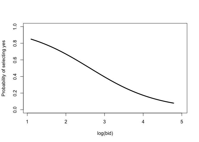
## Plot of probabilities of choosing yes is drawn as drawn as follows:
plot(NPdb)

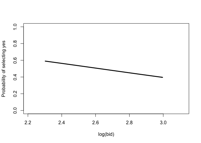
## The range of bid can be limited (e.g., [log(10), log(20)]):
plot(NPdb, bid = c(log(10), log(20)))

Created on 2020-01-16 by the reprex package (v0.3.0)
So, we at least know that the function will work on the NaturalPark data.
That does not guarantee, however, that it will work on all data.
Looking under the hood with
dbchoice
we find that it's a wrapper on optim
dbchoice <- optim(ini, fn = dbLL, method = "BFGS",
        hessian = TRUE, dvar = yvar, ivar = mmX, bid = bid, control = list(abstol = 10^(-30))))
This old S/O post explains the source of the problem, which is that when a zero value is passed to optim things fall apart.