See the FAQ: How to do a minimal reproducible example reprex for beginners for how to attract answers specific to your data.
Here's a good explainer on analysis of variance with an example using observation on three penguin species. It involves the use of the {dplyr} package to select rows. In {base} the same selection can be done with the subset operators [] where row is the first argument and column the second.
The example below is adapted from the explainer
library(ggplot2)
library(multcomp)
#> Loading required package: mvtnorm
#> Loading required package: survival
#> Loading required package: TH.data
#> Loading required package: MASS
#>
#> Attaching package: 'TH.data'
#> The following object is masked from 'package:MASS':
#>
#> geyser
library(palmerpenguins)
library(patchwork)
#>
#> Attaching package: 'patchwork'
#> The following object is masked from 'package:MASS':
#>
#> area
# remove row with NA and choose species and the two "bill_" variables
# not the fourth row, -4, and the first, third and fourth c(1,3,4))
opus <- penguins[-4,c(1,3,4)]
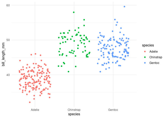
# recommended practice: visualize data
p1 <- ggplot(opus) +
aes(x = species, y = bill_length_mm, color = species) +
geom_jitter() +
theme(legend.position = "none") +
theme_minimal()
p2 <- ggplot(opus) +
aes(x = species, y = bill_length_mm, color = species) +
geom_boxplot() +
theme(legend.position = "none") +
theme_minimal()
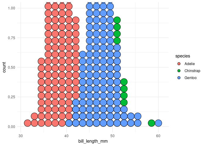
p3 <- ggplot(opus) +
aes(bill_length_mm, fill = species) +
geom_dotplot(method = "histodot", binwidth = 1.5) +
theme(legend.position = "none") +
theme_minimal()
p1
#> Warning: Removed 1 rows containing missing values (geom_point).
p2
#> Warning: Removed 1 rows containing non-finite values (stat_boxplot).

p3
#> Warning: Removed 1 rows containing non-finite values (stat_bindot).
res_aov <- aov(bill_length_mm ~ species, data = opus)
resids <- data.frame(.resid = res_aov$residuals)

# histogram
p4 <- ggplot(resids, aes(.resid)) +
  geom_histogram(color = "black", fill = "grey") +
  theme_minimal()

p5 <- ggplot(resids, aes(sample = .resid)) +
  stat_qq() +
  stat_qq_line() +
  theme_minimal()

p4 + p5
#> `stat_bin()` using `bins = 30`. Pick better value with `binwidth`.
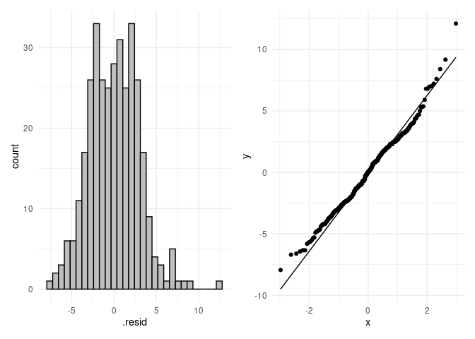
shapiro.test(res_aov$residuals)
#>
#> Shapiro-Wilk normality test
#>
#> data: res_aov$residuals
#> W = 0.98903, p-value = 0.01131
oneway.test(bill_length_mm ~ species,
data = opus,
var.equal = TRUE # assuming equal variances
)
#>
#> One-way analysis of means
#>
#> data: bill_length_mm and species
#> F = 410.6, num df = 2, denom df = 339, p-value < 2.2e-16
oneway.test(bill_length_mm ~ species,
data = opus,
var.equal = TRUE # assuming equal variances
)
#>
#> One-way analysis of means
#>
#> data: bill_length_mm and species
#> F = 410.6, num df = 2, denom df = 339, p-value < 2.2e-16
summary(res_aov)
#> Df Sum Sq Mean Sq F value Pr(>F)
#> species 2 7194 3597 410.6 <2e-16 ***
#> Residuals 339 2970 9
#> ---
#> Signif. codes: 0 '***' 0.001 '**' 0.01 '*' 0.05 '.' 0.1 ' ' 1
#> 1 observation deleted due to missingness
post_test <- glht(res_aov,
linfct = mcp(species = "Tukey")
)
summary(post_test)
#>
#> Simultaneous Tests for General Linear Hypotheses
#>
#> Multiple Comparisons of Means: Tukey Contrasts
#>
#>
#> Fit: aov(formula = bill_length_mm ~ species, data = opus)
#>
#> Linear Hypotheses:
#> Estimate Std. Error t value Pr(>|t|)
#> Chinstrap - Adelie == 0 10.0424 0.4323 23.232 < 0.001 ***
#> Gentoo - Adelie == 0 8.7135 0.3595 24.237 < 0.001 ***
#> Gentoo - Chinstrap == 0 -1.3289 0.4473 -2.971 0.00874 **
#> ---
#> Signif. codes: 0 '***' 0.001 '**' 0.01 '*' 0.05 '.' 0.1 ' ' 1
#> (Adjusted p values reported -- single-step method)
par(mar = c(3, 8, 3, 3))
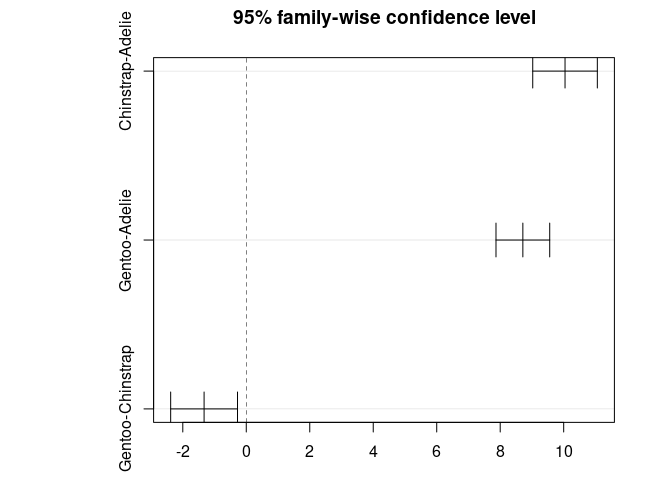
plot(post_test)
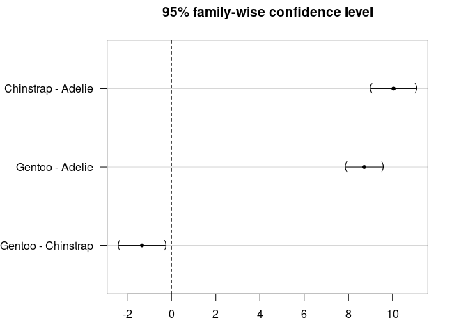
TukeyHSD(res_aov)
#>   Tukey multiple comparisons of means
#>     95% family-wise confidence level
#>
#> Fit: aov(formula = bill_length_mm ~ species, data = opus)
#>
#> $species
#>                       diff       lwr        upr     p adj
#> Chinstrap-Adelie 10.042433  9.024859 11.0600064 0.0000000
#> Gentoo-Adelie     8.713487  7.867194  9.5597807 0.0000000
#> Gentoo-Chinstrap -1.328945 -2.381868 -0.2760231 0.0088993

plot(TukeyHSD(res_aov))
Created on 2022-01-19 by the reprex package (v2.0.1)