NMDS: Non-metric multidimensional scaling ( NMDS ) is an indirect gradient analysis approach which produces an ordination based on a distance or dissimilarity matrix. ... Any dissimilarity coefficient or distance measure may be used to build the distance matrix used as input. NMDS is a rank-based approach.
I would like to obtain this analysis
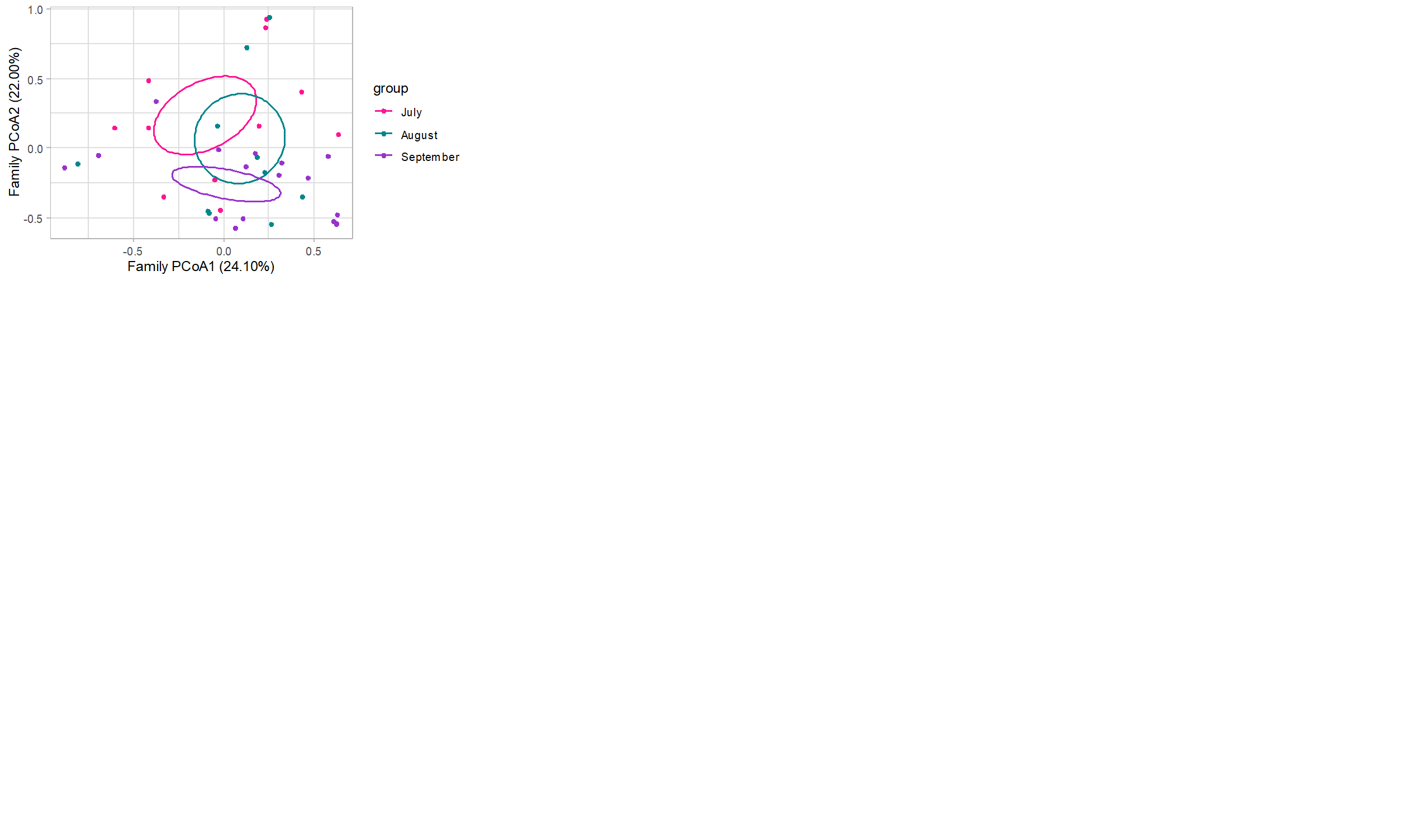
But with this differences

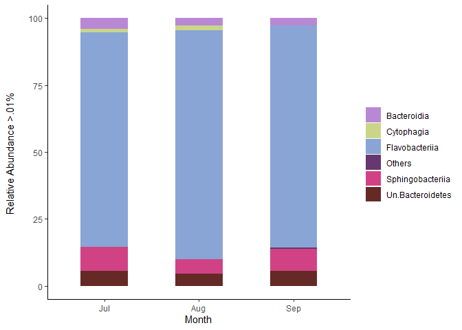
Two ellipses that cross each other means that there is similarity between them, when they do not cross each other, there are differences. As you can see in my barplot there are differences in the three months with respect to the microorganism communities.
And there are even more differences with respect to the month of August, and this is not being presented in the NMDS analysis.
I don't understand what your question is, I'm sorry.
Below is the correct barplot script, this is very summarized in information. I can't paste everything. So you can see that these differences were obtained because I first filtered per month.
library (tidyverse)
Family <-data.frame (tibble::tribble(
~index, ~Bacteroidia, ~Cytophagia, ~Flavobacteriia, ~Sphingobacteriia, ~Un.Bacteroidetes,
"1A", 7, 78, 5539, 255, 57,
"1B", 36, 4, 4820, 34, 33,
"1C", 32, 157, 453, 329, 64,
"1D", 0, 35, 1542, 113, 0,
"1E", 718, 90, 1975, 2401, 206,
"1F", 443, 204, 6944, 1704, 1671,
"1G", 49, 0, 2986, 34, 260,
"1H", 1040, 201, 10193, 351, 971,
"2A", 521, 231, 13510, 687, 504,
"2B", 845, 34, 8609, 299, 468,
"2C", 314, 38, 14687, 155, 68,
"2D", 24, 138, 2195, 759, 369,
"2E", 0, 70, 5734, 309, 10,
"2F", 668, 45, 7914, 464, 149,
"2G", 20, 141, 10438, 257, 154,
"2H", 168, 2, 12092, 954, 1459,
"3A", 1134, 639, 2613, 950, 1064,
"3B", 4, 0, 198, 33, 63,
"3C", 173, 18, 2493, 311, 48,
"3D", 0, 43, 2015, 41, 0,
"3E", 62, 14, 2434, 478, 72,
"3F", 346, 49, 3093, 339, 518,
"3G", 431, 80, 2655, 456, 618,
"3H", 25, 0, 481, 0, 19,
"4A", 1915, 345, 4426, 3228, 5273,
"4B", 0, 22, 13326, 280, 220,
"4C", 45, 0, 5156, 84, 50,
"4D", 46, 57, 4905, 824, 209,
"4E", 192, 126, 3572, 1135, 465,
"4F", 0, 0, 508, 0, 0,
"4G", 4, 187, 8384, 845, 13,
"4H", 1730, 52, 20979, 880, 5162,
"5A", 0, 15, 5376, 1091, 6,
"5B", 26, 842, 2095, 542, 337,
"5C", 0, 0, 124, 136, 42,
"5D", 260, 9, 7567, 88, 173,
"5E", 367, 74, 8499, 501, 341,
"5F", 556, 25, 11238, 522, 1159,
"5G", 0, 0, 45, 936, 77,
"5H", 0, 0, 6477, 1662, 22,
"6A", 478, 85, 14459, 833, 635,
"6B", 9, 115, 18826, 254, 60,
"6C", 152, 57, 3766, 412, 243,
"6D", 0, 95, 7290, 295, 19,
"6E", 135, 49, 2360, 1114, 299,
"6F", 300, 81, 8547, 828, 1113,
"6G", 0, 8, 2259, 4441, 0,
"6H", 2462, 371, 34631, 1635, 1046,
"7A", 0, 297, 4451, 482, 16,
"7B", 9, 371, 1463, 102, 9,
"7C", 127, 118, 3369, 82, 0,
"7D", 688, 218, 22223, 253, 223,
"7E", 1214, 37, 13024, 773, 731,
"7F", 806, 3, 12968, 39, 569,
"7G", 13, 0, 54, 50, 25,
"7H", 0, 0, 1271, 635, 0,
"8A", 577, 56, 13347, 765, 772,
"8B", 257, 149, 20001, 803, 1048,
"8C", 171, 37, 9434, 191, 195,
"8D", 355, 297, 3656, 2276, 794,
"8E", 856, 63, 2137, 467, 903,
"8F", 375, 117, 15910, 715, 778,
"8G", 65, 0, 371, 476, 292,
"8H", 149, 12, 12858, 519, 599,
"9A", 0, 609, 2101, 319, 116,
"9B", 289, 907, 4950, 1355, 590,
"9C", 0, 22, 1610, 0, 0,
"9D", 362, 710, 5405, 2516, 584,
"9E", 1281, 251, 17001, 978, 1097,
"9F", 456, 8, 42392, 1355, 1030,
"9G", 0, 13, 810, 1534, 194,
"9H", 371, 10, 2063, 440, 776,
"10A", 6, 98, 11000, 98, 58,
"10B", 23, 2, 13856, 100, 109,
"10C", 0, 36, 1650, 359, 105,
"10D", 213, 62, 10338, 73, 5,
"10E", 63, 10, 5733, 173, 50,
"10F", 106, 6, 10509, 278, 603,
"10G", 238, 4, 1506, 259, 304,
"10H", 32, 2, 2512, 170, 41,
"11A", 0, 12, 74, 0, 0,
"11B", 0, 0, 778, 0, 3,
"11C", 0, 62, 2852, 331, 32,
"11D", 261, 376, 2849, 1618, 554,
"11E", 310, 29, 7664, 458, 271,
"11F", 2, 141, 3557, 474, 0,
"11G", 0, 52, 1139, 424, 35,
"11H", 22, 203, 10735, 2474, 53,
"12A", 70, 11, 27508, 520, 406,
"12B", 636, 13, 9453, 448, 501,
"12C", 59, 8, 16805, 346, 430,
"12D", 63, 30, 223, 580, 956,
"12E", 6, 346, 6035, 304, 200,
"12F", 86, 63, 9172, 1041, 668,
"12G", 379, 42, 15882, 1723, 1842,
"12H", 385, 45, 25224, 2824, 1233
)
)
data<- Family
attach(Family)
rwnames <- index
data <- as.data.frame(data[,-1])
rownames(data) <- rwnames
Metadata<- data.frame (tibble::tribble(
~SampleID, ~SamplingPoint, ~Depth, ~Month,
"1A", "CEA1", "80 cm", "July",
"1B", "CEA2", "80 cm", "July",
"1C", "CEA4", "Interstitial", "July",
"1D", "CEA1", "80 cm", "August",
"1E", "CEA3", "80 cm", "August",
"1F", "CEA5", "80 cm", "August",
"1G", "CEA2", "80 cm", "September",
"1H", "CEA4", "80 cm", "September",
"2A", "CEA1", "80 cm", "July",
"2B", "CEA2", "Interstitial", "July",
"2C", "CEA4", "Interstitial", "July",
"2D", "CEA1", "80 cm", "August",
"2E", "CEA3", "80 cm", "August",
"2F", "CEA5", "80 cm", "August",
"2G", "CEA2", "80 cm", "September",
"2H", "CEA4", "80 cm", "September",
"3A", "CEA1", "Interstitial", "July",
"3B", "CEA2", "Interstitial", "July",
"3C", "CEA4", "80 cm", "July",
"3D", "CEA1", "Interstitial", "August",
"3E", "CEA3", "Interstitial", "August",
"3F", "CEA5", "Interstitial", "August",
"3G", "CEA2", "Interstitial", "September",
"3H", "CEA4", "Interstitial", "September",
"4A", "CEA1", "Interstitial", "July",
"4B", "CEA3", "80 cm", "July",
"4C", "CEA4", "Interstitial", "July",
"4D", "CEA1", "Interstitial", "August",
"4E", "CEA3", "Interstitial", "August",
"4F", "CEA5", "Interstitial", "August",
"4G", "CEA2", "Interstitial", "September",
"4H", "CEA4", "Interstitial", "September",
"5A", "CEA1", "80 cm", "July",
"5B", "CEA3", "80 cm", "July",
"5C", "CEA4", "Interstitial", "July",
"5D", "CEA1", "80 cm", "August",
"5E", "CEA3", "80 cm", "August",
"5F", "CEA5", "80 cm", "August",
"5G", "CEA2", "80 cm", "September",
"5H", "CEA4", "80 cm", "September",
"6A", "CEA1", "80 cm", "July",
"6B", "CEA3", "Interstitial", "July",
"6C", "CEA5", "80 cm", "July",
"6D", "CEA1", "80 cm", "August",
"6E", "CEA3", "Interstitial", "August",
"6F", "CEA5", "Interstitial", "August",
"6G", "CEA2", "Interstitial", "September",
"6H", "CEA4", "Interstitial", "September",
"7A", "CEA1", "Interstitial", "July",
"7B", "CEA3", "Interstitial", "July",
"7C", "CEA5", "80 cm", "July",
"7D", "CEA2", "80 cm", "August",
"7E", "CEA4", "80 cm", "August",
"7F", "CEA1", "80 cm", "September",
"7G", "CEA3", "80 cm", "September",
"7H", "CEA5", "80 cm", "September",
"8A", "CEA1", "Interstitial", "July",
"8B", "CEA3", "80 cm", "July",
"8C", "CEA5", "Interstitial", "July",
"8D", "CEA2", "80 cm", "August",
"8E", "CEA4", "80 cm", "August",
"8F", "CEA1", "80 cm", "September",
"8G", "CEA3", "80 cm", "September",
"8H", "CEA5", "80 cm", "September",
"9A", "CEA2", "80 cm", "July",
"9B", "CEA3", "Interstitial", "July",
"9C", "CEA5", "Interstitial", "July",
"9D", "CEA2", "Interstitial", "August",
"9E", "CEA4", "Interstitial", "August",
"9F", "CEA1", "Interstitial", "September",
"9G", "CEA3", "Interstitial", "September",
"9H", "CEA5", "Interstitial", "September",
"10A", "CEA2", "80 cm", "July",
"10B", "CEA3", "Interstitial", "July",
"10C", "CEA5", "80 cm", "July",
"10D", "CEA2", "Interstitial", "August",
"10E", "CEA4", "Interstitial", "August",
"10F", "CEA1", "Interstitial", "September",
"10G", "CEA3", "Interstitial", "September",
"10H", "CEA5", "Interstitial", "September",
"11A", "CEA2", "Interstitial", "July",
"11B", "CEA4", "80 cm", "July",
"11C", "CEA5", "Interstitial", "July",
"11D", "CEA2", "80 cm", "August",
"11E", "CEA4", "80 cm", "August",
"11F", "CEA1", "80 cm", "September",
"11G", "CEA3", "80 cm", "September",
"11H", "CEA5", "80 cm", "September",
"12A", "CEA2", "Interstitial", "July",
"12B", "CEA4", "80 cm", "July",
"12C", "CEA1", "Interstitial", "August",
"12D", "CEA2", "Interstitial", "August",
"12E", "CEA4", "Interstitial", "August",
"12F", "CEA1", "Interstitial", "September",
"12G", "CEA3", "Interstitial", "September",
"12H", "CEA5", "Interstitial", "September"
)
)
attach(Metadata)
rwnames <- SampleID
Metadata <- as.data.frame(Metadata[,-1])
rownames(Metadata) <- rwnames
#SUBSET DE MONTH
Jul <- subset(data, Metadata$Month == "July", select = c(`Bacteroidia`:`Un.Bacteroidetes`))
Aug <- subset(data, Metadata$Month == "August", select = c(`Bacteroidia`:`Un.Bacteroidetes`))
Sep <- subset(data, Metadata$Month == "September", select = c(`Bacteroidia`:`Un.Bacteroidetes`))
Metadata$Month <- factor(Metadata$Month,
levels = c("Jul", "Aug", "Sep"))
#July
Jul <- data.frame(Jul)
Jul_counts <- colSums(Jul)
Counts <- unname(Jul_counts)
Jul_counts <- data.frame(Jul_counts)
Jul_counts <- t(Jul_counts)
total <- sum(Counts)
rel_ab <- Jul_counts/total
Others <- rel_ab[,colMeans(rel_ab)<.01]
Others <- sum(Others)
rel_ab <- rel_ab[,colMeans(rel_ab)>=.01]
rel_ab <- data.frame(t(rel_ab), Others)
rel_ab_P <- t(rel_ab)
abundance <- c("abundance")
rel_ab_P <- data.frame(rel_ab_P)
write.csv(rel_ab_P, file = "~/RSTUDIO/Bacteria-total/Bacteria-total-clase_JUL_R.csv")
Jul <- read.csv("~/RSTUDIO/Bacteria-total/Bacteria-total-clase_JUL_R.csv")
#August
Aug <- data.frame(Aug)
Aug_counts <- colSums(Aug)
Counts <- unname(Aug_counts)
Aug_counts <- data.frame(Aug_counts)
Aug_counts <- t(Aug_counts)
total <- sum(Counts)
rel_ab <- Aug_counts/total
Others <- rel_ab[,colMeans(rel_ab)<.01]
Others <- sum(Others)
rel_ab <- rel_ab[,colMeans(rel_ab)>=.01]
rel_ab <- data.frame(t(rel_ab), Others)
rel_ab_P <- t(rel_ab)
abundance <- c("abundance")
rel_ab_P <- data.frame(rel_ab_P)
write.csv(rel_ab_P, file = "~/RSTUDIO/Bacteria-total/Bacteria-total-clase_AGU_R.csv")
Aug <- read.csv("~/RSTUDIO/Bacteria-total/Bacteria-total-clase_AGU_R.csv")
#September
Sep <- data.frame(Sep)
Sep_counts <- colSums(Sep)
Counts <- unname(Sep_counts)
Sep_counts <- data.frame(Sep_counts)
Sep_counts <- t(Sep_counts)
total <- sum(Counts)
rel_ab <- Sep_counts/total
Others <- rel_ab[,colMeans(rel_ab)<.01]
Others <- sum(Others)
rel_ab <- rel_ab[,colMeans(rel_ab)>=.01]
rel_ab <- data.frame(t(rel_ab), Others)
rel_ab_P <- t(rel_ab)
abundance <- c("abundance")
rel_ab_P <- data.frame(rel_ab_P)
write.csv(rel_ab_P, file = "~/RSTUDIO/Bacteria-total/Bacteria-total-clase_SEP_R.csv")
Sep <- read.csv("~/RSTUDIO/Bacteria-total/Bacteria-total-clase_SEP_R.csv")
Family_colors <- c(
"#b988d5","#cbd588", "#88a5d5",
"#673770","#D14285", "#652926", "#C84248",
"#8569D5", "#5E738F","#D1A33D", "#8A7C64", "#599861"
)
library(ggplot2)
library(scales)
#>
#> Attaching package: 'scales'
#> The following object is masked from 'package:purrr':
#>
#> discard
#> The following object is masked from 'package:readr':
#>
#> col_factor
ggplot() +geom_bar(aes(y = rel_ab_P*100, x= "Jul", fill = X), data = Jul,
stat="identity", width = .5)+ geom_bar(aes(y = rel_ab_P*100, x= "Aug", fill = X), data = Aug,
stat="identity",width=.5)+
scale_x_discrete(
labels = c("Jul", "Aug", "Sep"),
drop = FALSE
) +
geom_bar(aes(y = rel_ab_P*100, x= "Sep", fill = X), data = Sep,
stat="identity", width = .5)+
theme_classic()+
theme(legend.title = element_blank())+
ylab("Relative Abundance >.01% \n")+
xlab("Month")+
scale_fill_manual(values = Family_colors)
Created on 2020-03-04 by the reprex package (v0.3.0)