Because I've not really done much of it before, I thought I'd have a go at this for you.
Getting JSON Headlines
There's a Kaggle Dataset containing a million headlines from ABC News available as a .csv file here: A Million News Headlines | Kaggle
The code below augments the data with dates and randomly sampled names for authors from the babynames package. This tibble is then converted to JSON with toJSON and exported for analysis.
library("tidyverse")
library("lubridate")
library("babynames")
library("jsonlite")
library("here")

headlines_tib <- read_csv(here("abcnews-date-text.csv"))

headlines_tib <- headlines_tib %>%
  mutate(publish_date = ymd(publish_date)) %>%
  mutate(year = year(publish_date)) %>%
  mutate(authors = sample(babynames$name, nrow(.), replace = TRUE))

headlines_json <- toJSON(headlines_tib)

headlines_json %>%
  write_json("abcnews-headlines.json")
Importing JSON
Our dataset is contained in a single .json file that's 98Mb in size with 1.1million headlines. The read_json function will take a very long time to import this file. Fortunately, someone else on Community asked about importing very large JSON files here:
This code will stream in our file and then convert it from JSON into a nice tibble we can use. Note that I've used the tictoc package so you can time how long this process takes.
library("tictoc")
tic()
abc_news_headlines <- stream_in(file(here("abcnews-headlines.json")))
abc_news_headlines <- fromJSON(as.character(abc_news_headlines$V1))
toc()
Tagging headlines with categories
As I said at the top, I've not done much of this before. I leaned fairly heavily on this article:
We're going to use the udpipe package to extract and tally NOUN-VERB pairs in our dataset to identify potential categories. We'll only consider headlines from 2017 as I don't want to lock up my computer for longer than a coffee break. So we can join this dataset with others later on, I'm also adding a unique ID for each headline:
abc_news_2017 <- abc_news_headlines %>%
  filter(year == 2017) %>%
  mutate(headline_id = row_number())
To do this we need to download the latest version of our model, note that the filename changes after each update so ensure not to hard code the filename
library("udpipe")

model <- udpipe_download_model(language = "english")
file_udpipe <- list.files(pattern = ".udpipe")
udmodel_english <- udpipe_load_model(file = file_udpipe)
Now we annotate our headlines with udpipe_annotate() and convert the output into a tibble
tic()
annotations_headlines <- udpipe_annotate(udmodel_english, abc_news_2017$headline_text)
toc()
# 272.85 sec elapsed
headlines_annotated <- annotations_headlines %>%
  data.frame() %>%
  as_tibble()
Now we can extract our NOUN-VERB phrases using keywords_phrases()
headlines_annotated$phrase_tag <-
  as_phrasemachine(headlines_annotated$upos, type = "upos")
noun_verb_stats <-
  keywords_phrases(
    x = headlines_annotated$phrase_tag,
    term = tolower(headlines_annotated$token),
    pattern = "(A|N)*N(P+D*(A|N)*N)*",
    is_regex = TRUE,
    detailed = FALSE
  ) %>%
  as_tibble()
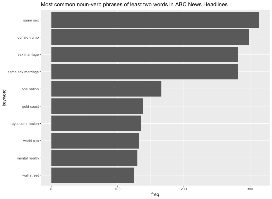
Let's look at the most common NOUN-VERB phrases, they definitely look suitable as categories:
noun_verb_stats %>%
  filter(ngram > 1) %>%
  filter(freq > 3) %>%
  arrange(desc(freq)) %>%
  slice(1:10) %>%
  mutate(keyword = fct_reorder(keyword, freq)) %>%
  ggplot(aes(x = keyword, y = freq)) +
  geom_col() +
  coord_flip() +
  labs(title = "Most common noun-verb phrases of least two words in ABC News Headlines")
Let's split our categories according to the number of words they contain:
two_word_topics <- noun_verb_stats %>%
  filter(ngram == 2) %>%
  filter(freq > 3) %>%
  select(keyword)

three_word_topics <- two_word_topics <- noun_verb_stats %>%
  filter(ngram == 3) %>%
  filter(freq > 3) %>%
  select(keyword)
The tidytext package now becomes really useful for us to detect our categories in the ngrams of our headlines:
tidy_two_word_topics <- abc_news_2017 %>%
  unnest_tokens(word, headline_text, token = "ngrams", n = 2) %>%
  filter(word %in% two_word_topics$keyword) %>%
  select(headline_id, word) %>%
  group_by(headline_id) %>%
  rename(two_word_topics = word) %>%
  mutate(two_word_topics = map(two_word_topics, ~list(.x))) %>%
  select(headline_id, two_word_topics) %>%
  mutate(n_two_word_topics = map_int(two_word_topics, ~length(.x))) %>%
  ungroup()

tidy_three_word_topics <- most_recent_headlines %>%
  unnest_tokens(word, headline_text, token = "ngrams", n = 3) %>%
  filter(word %in% three_word_topics$keyword) %>%
  select(headline_id, word) %>%
  group_by(headline_id) %>%
  rename(three_word_topics = word) %>%
  mutate(three_word_topics = map(three_word_topics, ~list(.x))) %>%
  select(headline_id, three_word_topics) %>%
  mutate(n_three_word_topics = map_int(three_word_topics, ~length(.x))) %>%
  ungroup()

tidy_topics <- tidy_two_word_topics %>%
  full_join(tidy_three_word_topics) %>%
  mutate(topics = pmap(list(two_word_topics, three_word_topics), ~c(.x, .y))) %>%
  mutate(n_topics = pmap_int(list(n_two_word_topics, n_three_word_topics), ~sum(.x, .y, na.rm = TRUE))) %>%
  select(headline_id, topics, n_topics)
Finally, we can rejoin this with our original headlines:
topiced_abc_news_2017 <- abc_news_2017 %>%
  full_join(tidy_topics) %>%
  filter(!is.na(n_topics)) %>%
  unnest(topics) %>%
  unnest(topics)

topiced_abc_news_2017 %>%
  head()
#> # A tibble: 6 x 7
#>   publish_date headline_text      year authors headline_id n_topics topics
#>   <date>       <chr>             <dbl> <chr>         <dbl>    <dbl> <chr>
#> 1 2017-01-01   ambulances ferry…  2017 Art               6        1 istanb…
#> 2 2017-01-01   manus island asy…  2017 Liesa            30        1 manus …
#> 3 2017-01-01   manus island asy…  2017 Liesa            30        1 island…
#> 4 2017-01-01   manus island asy…  2017 Ebb              31        1 manus …
#> 5 2017-01-01   manus island asy…  2017 Ebb              31        1 island…
#> 6 2017-01-01   north korea in f…  2017 Jeanet…          38        1 kim jo…
