You may want to read a bit on the subject; the process behind LISA (spatial lag, weights, Moran and local Moran) is heavy on theory.
But if your aim is to prepare a plot first, and improve on your understanding later - which is a perfectly legit aim! - you can consider something along these lines of code.
It relies heavily on {sfweight} package by Josh Parry, who might be active on this site. It provides a friendlier interface to older, and somewhat more general, but way more complex, {spdep} package. I am not certain if it is on CRAN at present, if not you can use the GitHub version.
As I don't have access to your data I am using the trusty old North Carolina shapefile that ships with {sf} package; you can easily replace it with your dataset.
You need to have three things in place before analyzing LISA clusters:
- spatial neighbors (read up on queen and rook approach; queen is the default); implemented via
sfweight::st_neighbors() - spatial weights, implemented via
sfweight::st_weights()with the neighbors as argument - spatial lag of a variable, implemented via
sfweight::st_lag(), with neigbors and weights as additional arguments
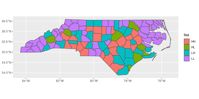
With these in place you can calculate the LISA categories using sfweight::categorize_lisa(), the arguments are your variable of interest and its spatial lag.
As I wrote, it is not the full story, but it should give you a start now to improve upon later...
library(sf)
library(dplyr)
library(sfweight) # remotes::install_github("Josiahparry/sfweight")
library(ggplot2)

shape <- st_read(system.file("shape/nc.shp", package="sf")) # included with sf package

# calucualte the lisa groups
shape_lisa <- shape %>%
  mutate(nb = st_neighbors(geometry),
         wts = st_weights(nb),
         lag_SID79 = st_lag(SID79, nb, wts),
         lisa = categorize_lisa(SID79, lag_SID79))

# report results
ggplot(data = shape_lisa) +
  geom_sf(aes(fill = lisa))