When melding two data frames like this
- Set the aesthetics in one and let the geoms inherit for it
mappingaesthetics for the other goes `aes(var1,var2), dat)- Make things simpler by using common variable names
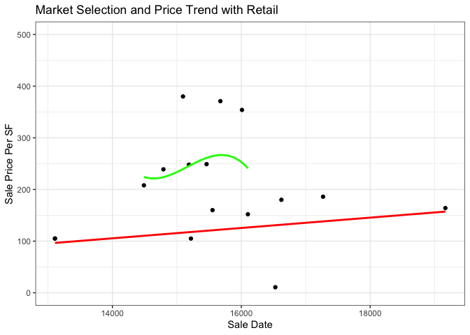
Any sequence of points can be connected to create a line that can be decomposed using a Fourier transform in the hope of extracting signal from noise. In the time series domain it is one tool to identify seasonality (recurrent patterns of consecutive events after removing trend and residuals). Where there is no true regularity in the occurrence of events beware of using linear fits, with or without polynomial transforms, there is danger of overfitting.
library(ggplot2)
library(ggthemes)
library(lubridate)
#>
#> Attaching package: 'lubridate'
#> The following objects are masked from 'package:base':
#>
#>     date, intersect, setdiff, union

juniors <- data.frame(
  Sale = c(
    2L, 6L, 20L, 24L, 25L, 37L, 42L, 55L,
    66L, 70L
  ),
  DateSale = c(
    "2009-09-01", "2010-07-01", "2011-05-01",
    "2011-08-01", "2011-09-01", "2012-05-01", "2012-08-01", "2012-12-01",
    "2013-11-01", "2014-02-01"
  ), Anchor = c(
    "Kohl's", "Kohl's", "Kohl's",
    "Kohl's", "JCPenny", "Forever", "Walmart", "Kohl's", "Kohl's",
    "Target"
  ), Center = c(
    "South Bay Galleria", "Elk Grove Commons",
    "Capitola Mall", "Parkway Plaza", "lhe Village At Orange", "2 i The atMontebello",
    "La Habra", "TheCrossroads At Pleasant Hill", "South Bay Galleria",
    "Northwood nSquare"
  ), SalePricePSF = c(
    208, 239, 380, 248, 105,
    249, 160, 371, 354, 152
  ), Overa = c(
    NA, 7.71, 6.58, NA, 6.02,
    6.29, 5.61, 6.75, 5.26, 6.1
  )
)

juniors$DateSale <- ymd(juniors$DateSale) |> as.integer()

head(juniors)
#>   Sale DateSale  Anchor                Center SalePricePSF Overa
#> 1    2    14488  Kohl's    South Bay Galleria          208    NA
#> 2    6    14791  Kohl's     Elk Grove Commons          239  7.71
#> 3   20    15095  Kohl's         Capitola Mall          380  6.58
#> 4   24    15187  Kohl's         Parkway Plaza          248    NA
#> 5   25    15218 JCPenny lhe Village At Orange          105  6.02
#> 6   37    15461 Forever  2 i The atMontebello          249  6.29

nordies <- read.csv("~/Desktop/grist.csv")
nordies$DateSaleT <- ymd(nordies$DateSaleT)
nordies
#>                   Address  DateSaleT SalePricePSFT PriceSaleT
#> 1     800 Coddingtown Ctr 2005-11-21         105.0   10562045
#> 2     900 Coddingtown Ctr 2005-11-21         105.0    7882123
#> 3    1363 N Mcdowell Blvd 2017-04-13         186.0   16416907
#> 4   8270 Petaluma Hill Rd 2015-04-03          10.8    1200000
#> 5 311 Rohnert Park Expy W 2022-06-24         164.0   14000000
#> 6      100 Santa Rosa Plz 2015-07-06         180.0   12829406

p <-
  juniors |> ggplot(aes(DateSale, SalePricePSF), fill = "green") +
  geom_point() +
  geom_smooth(method = "lm",
              formula = y ~ poly(x,3),
              se = F, color = "green") +
  geom_point(aes(DateSaleT,SalePricePSFT), nordies) +
  geom_smooth(aes(DateSaleT,SalePricePSFT),nordies, method = "lm",
              formula = y~poly(x,1),
              se = F, color = "red") +
  theme_economist() +
  coord_cartesian(ylim = c(0, 500)) +
  theme_bw()+
  labs(title = "Market Selection and Price Trend with Retail", x = "Sale Date", y = "Sale Price Per SF")

p
Created on 2023-01-26 with reprex v2.0.2