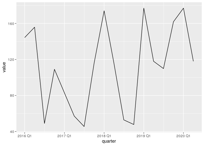
Your sample data doesn't have headers, and you have too many values per month, I still don't know to which time period they belong, I assume you have weekly data but I can't be sure so I'm going to arbitrarily reduce the data points just to exemplify how to perform time aggregation.
library(tidyverse)
library(lubridate)
library(tsibble)

TSpend <- data.frame(
    stringsAsFactors = FALSE,
    month = c("Jun","Aug","Sep","Aug",
              "Aug","Aug","Aug","Sep","Sep","Oct","Oct","Dec",
              "Dec","Dec","Feb","Jan","Feb","Feb","Mar","Mar","Apr",
              "Apr","May","May","May","Jun","May","Jun","Jun",
              "Aug","Dec","Feb","Jan","Mar","Mar","Apr","May",
              "May","Jun","Aug","Feb","Mar","Apr","Jun","Aug",
              "Feb","Jun","Aug","Feb","Aug","Aug","Mar","Feb",
              "Feb","Feb","Apr","Jan","Feb","May","Feb","Jan",
              "Feb","May","May","May","May","Oct","Jun","Jun",
              "Apr","Dec","Dec","Feb","Feb","Mar","Mar","Mar","Jan",
              "Jan","Jan","Nov","Nov","Nov","Nov","Feb","Feb",
              "Feb","Feb","Feb","Dec","Dec","Oct","Nov","May",
              "Jun","Jun","Jun","Jul","Jan","Jan","Mar","Mar",
              "Mar","May","Apr","Aug","Oct","Oct","Oct","Oct",
              "Jan","Jan","Feb","Feb","Feb","Feb","Jan","Jan",
              "Feb","Feb","Jan","Jan","Feb","Feb","Jan","Feb",
              "Jul","Nov","Nov","Apr","Apr","Apr","Apr","Apr","Sep",
              "Sep","Sep"),
    year = c("2019","2019","2019","2019",
             "2019","2019","2019","2019","2019","2019","2019",
             "2019","2019","2019","2020","2020","2020","2020",
             "2020","2020","2020","2020","2020","2020","2020",
             "2019","2019","2019","2019","2019","2019","2020",
             "2020","2020","2020","2020","2020","2019","2019",
             "2019","2020","2020","2020","2019","2019","2020",
             "2019","2019","2020","2019","2019","2019","2020","2020",
             "2020","2020","2019","2019","2019","2020","2019",
             "2019","2019","2019","2019","2019","2019","2018",
             "2018","2018","2017","2017","2018","2018","2018",
             "2018","2018","2018","2018","2018","2017","2017",
             "2017","2017","2018","2018","2018","2018","2018",
             "2017","2017","2016","2016","2016","2016","2017",
             "2017","2018","2016","2016","2016","2016","2016",
             "2016","2016","2016","2018","2018","2018","2018","2016",
             "2016","2016","2016","2016","2016","2016","2016",
             "2016","2016","2016","2016","2016","2016","2016",
             "2016","2017","2016","2019","2016","2016","2016",
             "2016","2016","2019","2019","2019"),
    value = c(59,59,59,59,59,59,59,59,
              59,59,59,59,59,59,59,59,59,59,59,59,59,59,
              59,59,59,59,59,59,59,59,59,59,59,59,59,59,
              59,59,59,59,59,59,59,59,59,59,59,59,59,59,59,
              59,59,59,59,59,59,59,59,59,59,59,59,59,59,
              59,59,58,58,58,58,58,58,58,58,58,58,58,58,
              58,58,58,58,58,58,58,58,58,58,58,58,57.66,
              57.66,57.12,57.12,57.12,57.12,52.91,51.06,51.06,
              51.06,51.06,51.06,51.06,51.06,48.99,47.78,47.78,
              47.78,47.78,46.1,46.1,46.1,46.1,46.1,46.1,46.1,46.1,
              46.1,46.1,46.1,46.1,46.1,46.1,46.1,46.1,45.54,
              45.16,43.91,43.33,43.33,43.33,43.33,43.33,42.8,
              42.8,42.8)
)

TSpend %>%
    group_by(year, month) %>%
    summarise(value = mean(value)) %>% # You have too many values per month I have to reduce them to exemplify
    mutate(date = dmy(paste0(01, month, year))) %>%
    as_tsibble(index = date) %>%
    index_by(quarter = ~ yearquarter(.)) %>%
    summarise(
        value = sum(value, na.rm = TRUE)
    ) %>%
    ggplot(aes(quarter, value)) +
    geom_line()

Created on 2020-09-01 by the reprex package (v0.3.0)